With the help of the Euler file povray.e, Euler can generate Povray files. The results are very nice to look at. For a detailed documentation have a look at the following page.
You need to load the povray file.
>load povray;
Make sure, the Povray bin directory is in the path. If it is not edit the following variable so that it contains the path to the povray executable.
>//defaultpovray="pvengine.exe"
For a first impression, we plot a simple function. The following command generates a povray file in your user directory, and runs Povray for ray tracing this file.
If you start the following command, the Povray GUI should open, run the file, and close automatically. Due to security reasons, you will be asked, if you want to allow the exe file to run. You can press cancel to stop further questions. You may have to press OK in the Povray window to acknowledge the start-up dialog of Povray.
>pov3d("x^2+y^2",zoom=3);
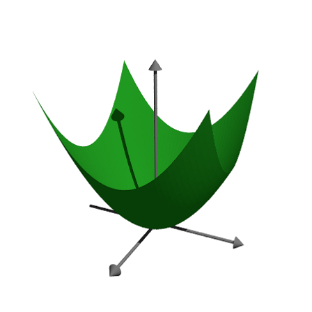
We can make the function transparent and add another finish. We can also add level lines to the function plot.
>pov3d("x^2+y^3",axiscolor=red,angle=20°, ...
   look=povlook(blue,0.2),level=-1:0.5:1,zoom=3.8);
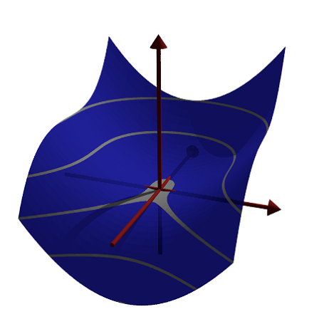
Sometimes it is necessary to prevent the scaling of the function, and scale the function by hand.
We plot the set of points in the complex plane, where the product of the distances to 1 and -1 is equal to 1.
>pov3d("((x-1)^2+y^2)*((x+1)^2+y^2)/40",r=1.5, ...
   angle=-120°,level=1/40,dlevel=0.005,light=[-1,1,1],height=45°,n=50, ...
   <fscale,zoom=3.8);
Instead of functions, we can plot with coordinates. As in plot3d, we need three matrices to define the object.
In the example we turn a function around the z-axis.
>function f(x) := x^3-x+1; ...
 x=-1:0.01:1; t=linspace(0,2pi,8)'; ...
 Z=x; X=cos(t)*f(x); Y=sin(t)*f(x); ...
 pov3d(X,Y,Z,angle=40°,height=20°,axis=0,zoom=4,light=[10,-5,5]);
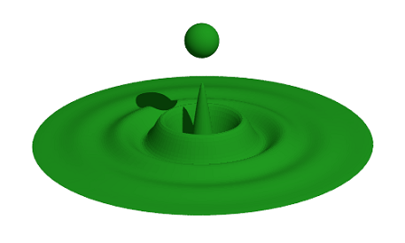
In the following example, we plot a damped wave. We generate the wave with the matrix language of Euler.
We also show, how an additional object can be added to a pov3d scene. For the generation of objects, see the following examples. Note that plot3d scales the plot, so that it fits into the unit cube.
>r=linspace(0,1,80); phi=linspace(0,2pi,80)'; ...
 x=r*cos(phi); y=r*sin(phi); z=exp(-5*r)*cos(8*pi*r)/3;  ...
 pov3d(x,y,z,zoom=5,axis=0,add=povsphere([0,0,0.5],0.1,povlook(green)), ...
   w=500,h=300);
With the advanced shading method of Povray, very few points can produce very smooth surfaces. Only at the boundaries and in shadows the trick might become obvious.
For this, we need to add normal vectors in each matrix point.
>Z &= x^2*y^3
                                 2  3
                                x  y
The equation of the surface is [x,y,Z]. We compute the two derivatives to x and y of this and take the cross product as the normal.
>dx &= diff([x,y,Z],x); dy &= diff([x,y,Z],y);
We define the normal as the cross product of these derivatives, and define coordinate functions.
>N &= crossproduct(dx,dy); NX &= N[1]; NY &= N[2]; NZ &= N[3]; N,
                               3       2  2
                       [- 2 x y , - 3 x  y , 1]
We use only 25 points.
>x=-1:0.5:1; y=x';
>pov3d(x,y,Z(x,y),angle=10°, ...
   xv=NX(x,y),yv=NY(x,y),zv=NZ(x,y),<shadow);
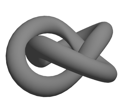
The following is the Trefoil knot done by A. Busser in Povray. There is an improved version of this in the examples.
For a good look with not too many points, we add normal vectors here. We use Maxima to compute the normals for us. First, the three functions for the coordinates as symbolic expressions.
>X &= ((4+sin(3*y))+cos(x))*cos(2*y); ...
 Y &= ((4+sin(3*y))+cos(x))*sin(2*y); ...
 Z &= sin(x)+2*cos(3*y);
Then the two derivative vectors to x and y.
>dx &= diff([X,Y,Z],x); dy &= diff([X,Y,Z],y);
Now the normal, which is the cross product of the two derivatives.
>dn &= crossproduct(dx,dy);
We now evaluate all this numerically.
>x:=linspace(-%pi,%pi,40); y:=linspace(-%pi,%pi,100)';
The normal vectors are evaluations of the symbolic expressions dn[i] for i=1,2,3. The syntax for this is &"expression"(parameters). This is an alternative to the method in the previous example, where we defined symbolic expressions NX, NY, NZ first.
>pov3d(X(x,y),Y(x,y),Z(x,y),axis=0,zoom=5,w=450,h=350, ...
   <shadow,look=povlook(gray), ...
   xv=&"dn[1]"(x,y), yv=&"dn[2]"(x,y), zv=&"dn[3]"(x,y));
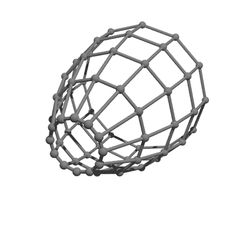
We can also generate a grid in 3D.
>povstart(zoom=4); ...
 x=-1:0.5:1; r=1-(x+1)^2/6; ...
 t=(0°:30°:360°)'; y=r*cos(t); z=r*sin(t); ...
 writeln(povgrid(x,y,z,d=0.02,dballs=0.05)); ...
 povend();
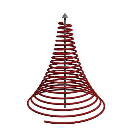
With povgrid(), curves are possible.
>povstart(center=[0,0,1],zoom=3.6); ...
 t=linspace(0,2,1000); r=exp(-t); ...
 x=cos(2*pi*10*t)*r; y=sin(2*pi*10*t)*r; z=t; ...
 writeln(povgrid(x,y,z,povlook(red))); ...
 writeAxis(0,2,axis=3); ...
 povend();
Above, we used pov3d to plot surfaces. The povray interface in Euler can also generate Povray objects. These objects are stored as strings in Euler, and need to be written to a Povray file.
We start the output with povstart().
>povstart(zoom=4);
First we define the three cylinders, and store them in strings in Euler.
The functions povx() etc. simply returns the vector [1,0,0], which could be used instead.
>c1=povcylinder(-povx,povx,1,povlook(red)); ...
 c2=povcylinder(-povy,povy,1,povlook(green)); ...
 c3=povcylinder(-povz,povz,1,povlook(blue)); ...
The strings contain Povray code, which we need not understand at that point.
>c1
cylinder { <-1,0,0>, <1,0,0>, 1
 texture { pigment { color rgb <0.564706,0.0627451,0.0627451> }  }
 finish { ambient 0.2 }
 }
As you see, we added texture to the objects in three different colors.
That is done by povlook(), which returns a string with the relevant Povray code. We can use the default Euler colors, or define our own color. We can also add transparency, or change the ambient light.
>povlook(rgb(0.1,0.2,0.3),0.1,0.5)
 texture { pigment { color rgbf <0.101961,0.2,0.301961,0.1> }  }
 finish { ambient 0.5 }
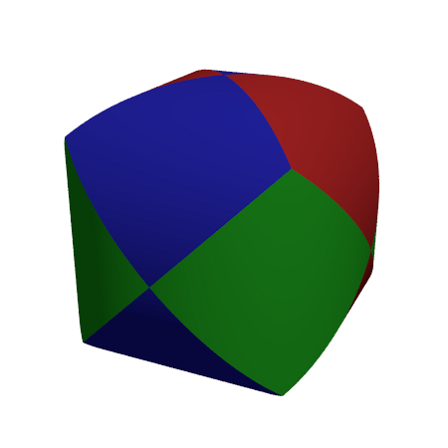
Now we define an intersection object, and write the result to the file.
>writeln(povintersection([c1,c2,c3]));
The intersection of three cylinders is hard to visualize, if you never saw it before.
>povend;
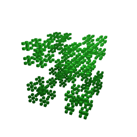
The following functions generate a fractal recursively.
The first function shows, how Euler handles simple Povray objects. The function povbox() returns a string, containing the box coordinates, the texture and the finish.
>function onebox(x,y,z,d) := povbox([x,y,z],[x+d,y+d,z+d],povlook());
>function fractal (x,y,z,h,n) ...
  if n==1 then writeln(onebox(x,y,z,h));
  else
    h=h/3;
    fractal(x,y,z,h,n-1);
    fractal(x+2*h,y,z,h,n-1);
    fractal(x,y+2*h,z,h,n-1);
    fractal(x,y,z+2*h,h,n-1);
    fractal(x+2*h,y+2*h,z,h,n-1);
    fractal(x+2*h,y,z+2*h,h,n-1);
    fractal(x,y+2*h,z+2*h,h,n-1);
    fractal(x+2*h,y+2*h,z+2*h,h,n-1);
    fractal(x+h,y+h,z+h,h,n-1);
  endif;
 endfunction
>povstart(fade=10,<shadow);
>fractal(-1,-1,-1,2,4);
>povend();
Differences allow cutting off one object from another. Like intersections, there are part of the CSG objects of Povray.
>povstart(light=[5,-5,5],fade=10);
For this demonstration, we define an object in Povray, instead of using a string in Euler. Definitions are written to the file immediately.
A box coordinate of -1 just means [-1,-1,-1].
>povdefine("mycube",povbox(-1,1));
We can use this object in povobject(), which returns a string as usual.
>c1=povobject("mycube",povlook(red));
We generate a second cube, and rotate and scale it a bit.
>c2=povobject("mycube",povlook(yellow),translate=[1,1,1], ...
   rotate=xrotate(10°)+yrotate(10°), scale=1.2);
Then we take the difference of the two objects.
>writeln(povdifference(c1,c2));
Now add three axes.
>writeAxis(-1.2,1.2,axis=1); ...
 writeAxis(-1.2,1.2,axis=2); ...
 writeAxis(-1.2,1.2,axis=4); ...
 povend();
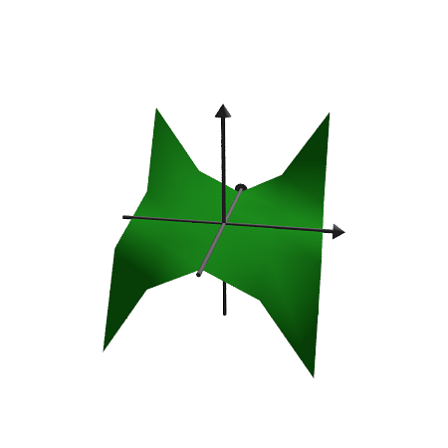
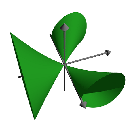
Povray can plot the set where f(x,y,z)=0, just like the implicit parameter in plot3d. The results looks much better, however.
The syntax for the functions is a bit different. You cannot use the output of Maxima or Euler expressions.
>povstart(angle=70°,height=50°,zoom=4);
Create the implicit surface. Note the different syntax in the expression.
>writeln(povsurface("pow(x,2)*y-pow(y,3)-pow(z,2)",povlook(green))); ...
 writeAxes(); ...
 povend();
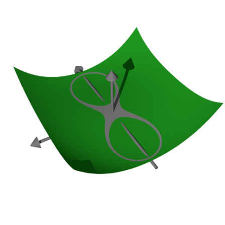
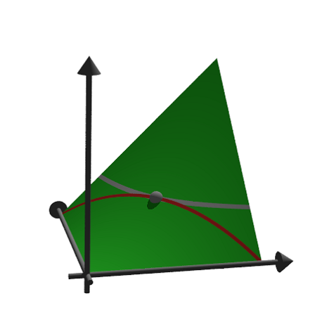
In this example, we show how to create a mesh object, and draw it with additional information.
We like to maximize xy under the condition x+y=1 and demonstrate the tangential touching of the level lines.
>povstart(angle=-10°,center=[0.5,0.5,0.5],zoom=7);
We cannot store the object in a string as before, since is too large. So we define the object in a Povray file using #declare. The function povtriangle() does this automatically. It can accept normal vectors just like pov3d().
The following defines the mesh object, and writes it immediately into the file.
>x=0:0.02:1; y=x'; z=x*y; vx=-y; vy=-x; vz=1;
>mesh=povtriangles(x,y,z,"",vx,vy,vz);
Now we define two discs, which will be intersected with the surface.
>cl=povdisc([0.5,0.5,0],[1,1,0],2); ...
 ll=povdisc([0,0,1/4],[0,0,1],2);
Write the surface minus the two discs.
>writeln(povdifference(mesh,povunion([cl,ll]),povlook(green)));
Write the two intersections.
>writeln(povintersection([mesh,cl],povlook(red))); ...
 writeln(povintersection([mesh,ll],povlook(gray)));
Write a point at the maximum.
>writeln(povpoint([1/2,1/2,1/4],povlook(gray),size=2*defaultpointsize));
Add axes and finish.
>writeAxes(0,1,0,1,0,1,d=0.015); ...
 povend();
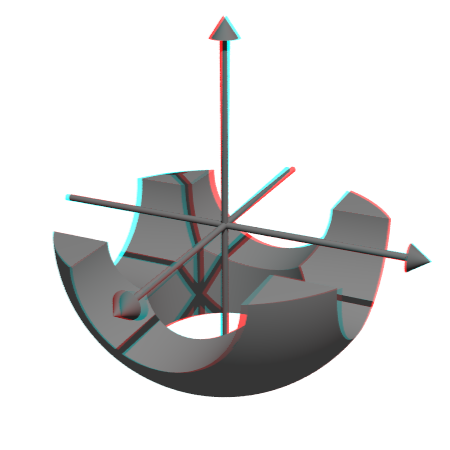
To generate an anaglyph for a red/cyan glasses, Povray must run twice from different camera positions. It generates two Povray files and two PNG files, which are loaded with the function loadanaglyph().
Of course, you need red/cyan glasses to view the following examples properly.
The function pov3d() has a simple switch to generate anaglyphs.
>pov3d("-exp(-x^2-y^2)/2",r=2,height=45°,>anaglyph, ...
   center=[0,0,0.5],zoom=3.5);

If you create a scene with objects, you need to put the generation of the scene into a function, and run it twice with different values for the anaglyph parameter.
>function myscene ...
   s=povsphere(povc,1);
   cl=povcylinder(-povz,povz,0.5);
   clx=povobject(cl,rotate=xrotate(90°));
   cly=povobject(cl,rotate=yrotate(90°));
   c=povbox([-1,-1,0],1);
   un=povunion([cl,clx,cly,c]);
   obj=povdifference(s,un,povlook(red));
   writeln(obj);
   writeAxes();
 endfunction
The function povanaglyph() does all this. The parameters are like in povstart() and povend() combined.
>povanaglyph("myscene",zoom=4.5);
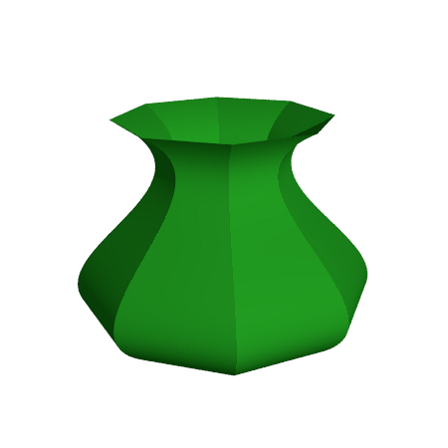
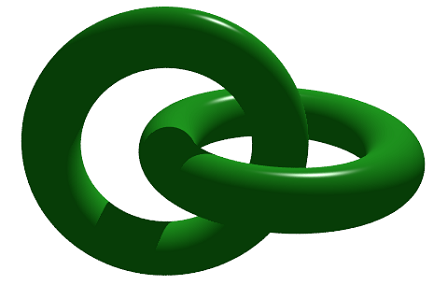
The povray interface of Euler contains a lot of objects. But you are not restricted to these. You can create own objects, which combine other objects, or are completely new objects.
We demonstrate a torus. The Povray command for this is "torus". So we return a string with this command and its parameters. Note that the torus is always centered at the origin.
>function povdonat (r1,r2,look="") ...
   return "torus {"+r1+","+r2+look+"}";
 endfunction
Here is our first torus.
>t1=povdonat(0.8,0.2)
torus {0.8,0.2}
Let us use this object to create a second torus, translated and rotated.
>t2=povobject(t1,rotate=xrotate(90°),translate=[0.8,0,0])
object { torus {0.8,0.2}
 rotate 90 *x
 translate <0.8,0,0>
 }
Now we place these objects into a scene. For the look, we use Phong Shading.
>povstart(center=[0.4,0,0],angle=0°,zoom=3.8,aspect=1.5); ...
 writeln(povobject(t1,povlook(green,phong=1))); ...
 writeln(povobject(t2,povlook(green,phong=1))); ...
>povend();
calls the Povray program. However, in case of errors, it does not display the error. You should therefore use
>povend(<exit);
if anything did not work. This will leave the Povray window open.
>povend(h=320,w=480);
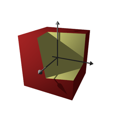
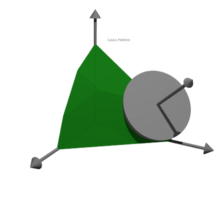
Here is a more elaborate example. We solve
![]()
and show the feasible points and the optimum in a 3D plot.
>A=[10,8,4;5,6,8;6,3,2;9,5,6];
>b=[10,10,10,10]';
>c=[1,1,1];
First, let us check, if this example has a solution at all.
>x=simplex(A,b,c,>max,>check)'
[0, 1, 0.5]
Yes, it has.
Next we define two objects. The first is the plane
![]()
>function oneplane (a,b,look="") ...
   return povplane(a,b,look)
 endfunction
Then we define the intersection of all half spaces and a cube.
>function adm (A, b, r, look="") ...
   ol=[];
   loop 1 to rows(A); ol=ol|oneplane(A[#],b[#]); end;
   ol=ol|povbox([0,0,0],[r,r,r]);
   return povintersection(ol,look);
 endfunction
We can now plot the scene.
>povstart(angle=120°,center=[0.5,0.5,0.5],zoom=3.5); ...
 writeln(adm(A,b,2,povlook(green,0.4))); ...
 writeAxes(0,1.3,0,1.6,0,1.5); ...
The following is a circle around the optimum.
>writeln(povintersection([povsphere(x,0.5),povplane(c,c.x')], ...
   povlook(red,0.9)));
And an error in the direction of the optimum.
>writeln(povarrow(x,c*0.5,povlook(red)));
We add text to the screen. Text is just a 3D object. We need to place and turn it according to our view.
>writeln(povtext("Linear Problem",[0,0.2,1.3],size=0.05,rotate=125°)); ...
 povend();
You can find some more examples for Povray in Euler in the following files.
Examples/Dandelin Spheres
Examples/Donat Math
Examples/Trefoil Knot
Examples/Optimization by Affine Scaling