This is a short introduction to Maxima for Euler. For more information on Maxima view their homepage at SourceForge, or the reference delivered and installed with Euler.
Maxima Homepage
Maxima Reference
Syntax of Euler
More detailed Tutorial for Maxima
For internals about the communication between Euler and Maxima see the last section.
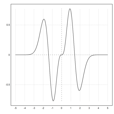
The preferred method to use Maxima in Euler are symbolic expressions and functions. Symbolic expressions start with "&" and can be used at any place in Euler where expressions are allowed. In the following, we plot
![]()
>plot2d(&diff(x^4*exp(-x^2),x),-5,5):
Symbolic expressions are evaluated by Maxima. The result is printed by Maxima as a display formula.
>&diff(x^4*exp(-x^2),x)
                                2            2
                          3  - x       5  - x
                       4 x  E     - 2 x  E
If Latex is installed properly, the result can be displayed using Latex with $...
>$factor(diff(x^4*exp(-x^2),x))
![]()
The symbolic expression is scanned by Euler to determine the expression for Maxima. You can help Euler with quotes, if needed. The quotes are necessary, if symbolic expressions are computed in Euler functions at run time.
>&"factor(x/7+y*(x/5+x/9))"
                            x (98 y + 45)
                            -------------
                                 315
Symbolic expressions can be stored in variables using &=.
>fx &= log(x)/x
                                log(x)
                                ------
                                  x
It helps to be aware that the symbolic variable fx is defined for Euler in a string, which prints as a symbolic expression.
>fx
                                log(x)
                                ------
                                  x
To see that the expression behaves like a string, we concatenate it to an Euler string.
>"Expression: "+fx
Expression: log(x)/x
The expression is stored in Maxima in a symbolic variable, which can be used in other symbolic expressions.
>&fx^2
                                  2
                               log (x)
                               -------
                                  2
                                 x
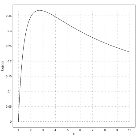
You can plot the expression in Euler as usual. This works because the function is just an expression in x, stored in a string.
>plot2d(fx,1,10,xl="x",yl="log(x)/x"):
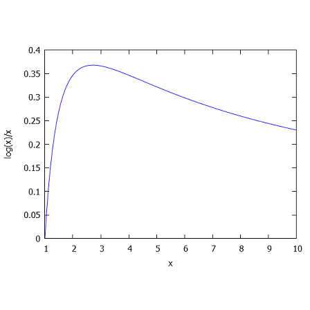
You can also use Gnuplot for this. Read more about Gnuplot below.
>&plot2d(fx,[x,1,10]):
In the following command, "solve" is the numerical Euler function "solve", not the symbolic solver, solving
![]()
close to 3. We pass an expression to solve(), which has been computed by Maxima. The start value 3 for the numerical algorithm is needed.
>solve(&diff(fx,x),3)
2.71828182846
For the simple function fx, we can also call Maxima to solve the value exactly. For this, we let Maxima evaluate "solve(diff(fx,x))".
>&solve(diff(fx,x))
[x = E]
We can also apply other numerical methods to the expression.
>romberg(&fx,1,E)
0.5
This is indeed the correct integral. Maxima can compute the integral for this simple function exactly.
>&integrate(fx,x,1,E)
                                  1
                                  -
                                  2
You can easily define an expression for the second derivative. The right hand side of &= is parsed through Maxima before the definition.
>d2fx &= factor(diff(fx,x,2))
                             2 log(x) - 3
                             ------------
                                   3
                                  x
To find the the turning point numerically, use the numerical solver.
>solve(d2fx,E,4)
4.48168907034
An exact solution is possible in this case.
>&solve(d2fx,x)
                                    3/2
                              [x = E   ]
Like symbolic expressions, you can define a symbolic function. The function definition uses &= in this case.
The right hand side is evaluated in Maxima before the definition of the function. In the following example, it simply calls the symbolic expression fx.
>function f(x) &= fx
                                log(x)
                                ------
                                  x
The function can be used in a symbolic way or numerically.
>&f(x+1), f(4),
                              log(x + 1)
                              ----------
                                x + 1

0.34657359028
Here is a function for the tangent line of f in x0.
>function T(x,x0) &= f(x0)+(x-x0)*diffat(f(x),x=x0)
                             1    log(x0)    log(x0)
                  (x - x0) (--- - -------) + -------
                              2       2        x0
                            x0      x0
The function diffat() is an extension of Euler to the syntax of Maxima (see below).
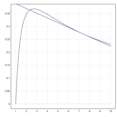
Let us plot the function and its tangent in one plot.
>plot2d("f(x)",1,10); plot2d("T(x,E^(4/2))",add=1,color=4):
If you tried to find a tangent function, which goes through the point (0,-2), you would fail in Maxima. There is no closed solution for this.
>&solve(T(0,x)=-2,x)
                               1 - 2 log(x)
                          [x = ------------]
                                    2
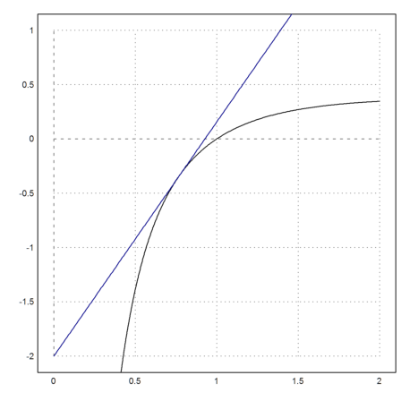
However, in Euler you can easily find a numerical solution.
>x0 := solve(&T(0,x),1,y=-2)
0.766248608162
>plot2d("f(x)",0,2,-2,1); plot2d("T(x,x0)",add=1,color=4):
If you look at a symbolic function, you see that the expression returned by Maxima is inserted into an Euler function for numerical evaluation.
>type f
function f (x)
useglobal; return log(x)/x
endfunction
This can be done for multi-line functions too. We refer to the tutorial about programming for more details.
Maxima has a numerical library like Euler.
>&float(exp(2))
7.38905609893065
But for Euler, the result is a string. If you need the value in Euler, you need to evaluate this string. This can be done by the usual evaluation mechanism expression() of Euler. In the example we quote the symbolic expression explicitly.
>log(&float(exp(2))())
2
This mechanism for evaluation can be used for any symbolic expression.
>expr &= x^3-x+1
                               3
                              x  - x + 1
The evaluation works just like for Euler expressions. The variable x must be globally known or given as a parameter. Note that unnamed parameters are assigned to x, y, z automatically.
>expr(5)
121
Thus you need not define a symbolic function. Instead, evaluate the expression.
>expr &= taylor(exp(x^2+a),x,0,5), expr(0.2,a=2)
                           a  4
                          E  x     a  2    a
                          ----- + E  x  + E
                            2

7.69052958777
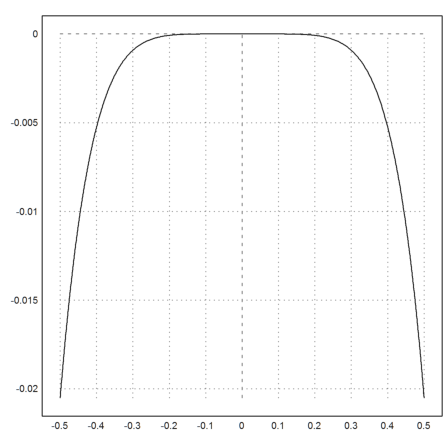
You can use the expression just like a function.
>plot2d("expr(x,a=2)-exp(x^2+2)",-0.5,0.5):
A special feature of the evaluation will evaluate solutions from the symbolic solver. The variables "x=" etc. are skipped.
>&solve(x^2+x+1), %()
                    - sqrt(3) I - 1      sqrt(3) I - 1
               [x = ---------------, x = -------------]
                           2                   2

[ -0.5-0.866025i,  -0.5+0.866025i ]
If you have a variable with a numerical value in Euler, it can be inserted into an expression for Maxima with @name.
>x=3; &a+@x
a + 3
Thus you can evaluate a Maxima function with a numerical value from Euler, without setting a variable in Maxima.
One useful example for this method are evaluations with big float in Maxima.
>x=3; &bfloat(exp(@x))
2.0085536923187667740928529654582b1
Another useful application are functions, which are not implemented in Euler. For an example, we load the distribution package in Maxima.
>&load(distrib);
There is a function called the incomplete exponential integral.
>&expintegral_ei(2.0)
4.95423435600189
It is defined as
![]()
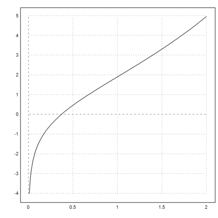
We can make this an Euler function, using the evaluation of Maxima. This will be a bit slow, but it works.
>function map expintegralInMaxima(x) := &"float(expintegral_ei(@x))"()
We need to vectorize the function with map, since Maxima cannot evaluate its functions for vectors. But now we apply the function to vectors.
>t=0.01:0.01:2; s=expintegralInMaxima(t); plot2d(t,s):
The exponential integral has the following representation in a series.
![]()
Thus it can be evaluated for reasonable small values of x in the following way. We first define the truncated series as a polynomial.
>eipol := gamma$|1/((1:20)!*(1:20))
[0.577216,  1,  0.25,  0.0555556,  0.0104167,  0.00166667,
0.000231481,  2.83447e-005,  3.1002e-006,  3.06192e-007,
2.75573e-008,  2.27746e-009,  1.73973e-010,  1.23531e-011,
8.19339e-013,  5.09811e-014,  0,  0,  0,  0,  0]
Now we define a numerical function for Euler.
If we want to give the function the same name as the Maxima function, we need to use the double underscore in Euler.
>function expintegral__ei(x) := evalpoly(x,eipol)+log(abs(x));
The error is small. We compare the evaluation of Maxima and our series for a vector of values.
>t=0.01:0.01:2; max(abs(expintegralInMaxima(t)-expintegral__ei(t)))
0
A special feature of the Maxima interface is that _ is replaced by __ for Euler. Maxima would not understand the double underscore, and Euler would interpret the single underscore as the vertical concatenation.
Thus the following evaluation works as expected. Note that the evaluation uses the numerical series of Euler!
>&expintegral_ei(2); ""+%, %()
expintegral__ei(2)
4.954234356
For a symbolic expression, _ is replaced by __ too.
>expr &= expintegral_ei(x)
expintegral_ei(x)
You can see this only, if you print the expression as an Euler string.
>""|expr
expintegral__ei(x)
Now the expression can evaluate in Euler and in Maxima.
>longest expr(2), &expr with x=2.0
      4.954234356001888

                           4.95423435600189
Another way to use Maxima in Euler is to send commands directly to the Maxima system, which runs as a process and communicates with Euler. Append "::" or ":::" in front of the command to send it to Maxima.
":: " is the compatibility mode
"::: " sends the command verbatim to Maxima
The compatibility mode makes the Maxima syntax similar to the Euler syntax. E.g., it uses ":=" to set variables instead of ":", and uses ";" to separate commands and not print results, and "," to print results, just as Euler does. The direct mode is for experts in Maxima.
>:: 30!, factor(%)
                  265252859812191058636308480000000


                   26  14  7  4   2   2
                  2   3   5  7  11  13  17 19 23 29
With "%", it is possible to refer to the previous output, just as in Euler. However, to access results over several lines it is better to use variables.
As in Euler, "//" starts a comment.
A line can contain several Maxima commands. The commands are sent to Maxima one after the other. Separate the commands with "," or with ";".
>:: expand((1+x)^10), factor(diff(%,x))
         10       9       8        7        6        5        4
        x   + 10 x  + 45 x  + 120 x  + 210 x  + 252 x  + 210 x
                                                  3       2
                                           + 120 x  + 45 x  + 10 x + 1


                                       9
                             10 (x + 1)
In case, you wish to use the direct mode, remember that "$" suppresses the output of a command, ":" is used to set variables, and "," is used for flags to a command. The delimiter ";" prints the output of a command.
By default the direct mode is disabled. But with "::: ...", you can call it nevertheless. If you enable the direct mode ": ..." can be used for this mode.
>::: expr:1+x$ (1+x)^10; %,expand
                                     10
                              (x + 1)


         10       9       8        7        6        5        4
        x   + 10 x  + 45 x  + 120 x  + 210 x  + 252 x  + 210 x
                                                  3       2
                                           + 120 x  + 45 x  + 10 x + 1
As you see, the syntax is quite different from the compatible syntax. You might need the direct mode if you are reading a book about Maxima and want to try the examples in Euler.
>::: define(fh(x),diff(x*exp(x),x));
                                      x    x
                          fh(x) := x E  + E
>::: fh(5);
                                    5
                                 6 E
It is also possible to switch to Maxima mode permanently. All commands are Maxima commands from that point on. Euler can be configured to start in Maxima mode automatically.
We use this mode to demonstrate some features of Maxima.
>maximamode on
Maxima mode is on (compatibility mode)
The default mode is the compatibility mode. But you also use the direct mode with
>maximamode direct
Note that variables are set with := in Maxima. Here we set a=3, then evaluate an expression in a, then kill the variable a.
>a:=3; (1+a)^3, remvalue(a);
64
Another way to evaluate an expression with a value is to locally set the variable. The flag "with ..." does this. Append it to the command.
>(1+a)^3 with a=3
64
The third method to evaluate an expression with a value is to define a Maxima function.
>function f(a) := (1+a)^3
                                          3
                           f(a) := (1 + a)
>f(3)
64
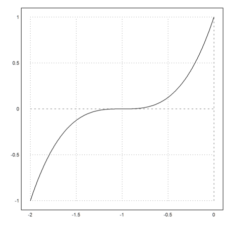
You can send commands to Euler in this mode too. Note that f has been defined for Maxima only. So we use a symbolic expression to get f(x) for Euler.
>euler plot2d(&f(x),-2,0):
Maxima does not automatically simplify completely. You need to say, what you want. In the following example, we go back and forth from one form to another of a rational expression.
Remember, that we are still in Maxima mode.
>2/a + a + 1/a^2, factor(%), expand(%)
                                  2   1
                              a + - + --
                                  a    2
                                      a


                              3
                             a  + 2 a + 1
                             ------------
                                   2
                                  a


                                  2   1
                              a + - + --
                                  a    2
                                      a
Another way to simplify a rational function is to apply the command "ratsimp" to the evaluation.
Such flags have to be appended using | ...
>2/a + a + 1/a^2 | ratsimp
                              3
                             a  + 2 a + 1
                             ------------
                                   2
                                  a
Appending the command after a "|" is equivalent to a direct command for many simplifications.
>ratsimp(2/a+a+1/a^2)
                              3
                             a  + 2 a + 1
                             ------------
                                   2
                                  a
"ratsimp" and "factor" will also cancel common factors in the numerator and denominator.
>(a^3+3*a+3*a^2+1)/(a+1), factor(%)
                          3      2
                         a  + 3 a  + 3 a + 1
                         -------------------
                                a + 1


                                      2
                               (a + 1)
Some other commands can simplify more complex expressions. You might want to try "radcan" and "trigsimp".
>radcan(log(100)/log(10))
2
>trigsimp(sin(x)^2+cos(x)^2)
1
"simpsum" is a command, which simplifies and evaluates a sum.
>sum(k^2,k,1,n) | simpsum | factor
                         n (n + 1) (2 n + 1)
                         -------------------
                                  6
Of course, Maxima can differentiate and integrate too.
We are still in Maxima mode.
>diff(x^x,x)
                            x
                           x  (log(x) + 1)
Here is the second derivative.
>diff(x^x,x,2)
                       x             2    x - 1
                      x  (log(x) + 1)  + x
You can use "at" to evaluate the derivative at a specific point.
>at(diff(x^x,x,2),x=1)
2
A nicer way to set a value or several values is the "with" operator, which is added to Maxima by Euler.
>diff(x^x,x,2) with x=1
2
However, it might be easier to use the function "diffat", which is an extension of Maxima in Euler.
>diffat(x^x,x=1,2)
2
Other derivatives are gradient(), grad(), hessian() and jacobian(). These functions return Maxima matrices. See below for more information.
>gradient(x^y,[x,y])
                          y - 1     y
                        [x      y, x  log(x)]
You can use grad(), if there are no other variables involved.
>grad(x^y)
                          y - 1     y
                        [x      y, x  log(x)]
>hessian(x^2+y^2+x*y,[x,y])
                               [ 2  1 ]
                               [      ]
                               [ 1  2 ]
>jacobian([x^y,y^x],[x,y])
                       [  y - 1      y        ]
                       [ x      y   x  log(x) ]
                       [                      ]
                       [  x            x - 1  ]
                       [ y  log(y)  x y       ]
If you are in a hurry, omit the variable list, using grad(f) or hesse(f).
>grad(x^2+y^2)
[2 x, 2 y]
For the following, we switch off Maxima mode.
>maximamode off
Maxima mode is off
Since strings, which contain expressions in x can be evaluated at specific values of x, this makes the evaluation of a Maxima result easy.
We are back in Euler mode.
>&diff(x^x,x,2)(4)
1521.76659915
Alternatively, the string can be evaluated with global values.
>x:=4; &diff(x^x,x,2)()
1521.76659915
There is a shortcut for this. &:expression evaluates the expression and uses the result directly as an Euler command.
>x:=4; &:diff(x^x,x,2)
1521.76659915
Alternatively, we can store the expression into variables of Euler and Maxima, and evaluate later.
>x:=4; expr &= diff(x^x,x,2); expr()
1521.76659915
The symbolic gradient function returns a symbolic vector.
>&gradient(x^2-y^2,[x,y])
[2 x, - 2 y]
The numerical value of the Hessian matrix is computed by mxmhessian. We evaluate the result at x=y=E.
>&hessian(x^y-y^x,[x,y])(E,E)
     -5.57494             0
            0       5.57494
The same method works for integrals.
>&integrate(x*sin(x),x,0,1), %()
                           sin(1) - cos(1)

0.30116867894
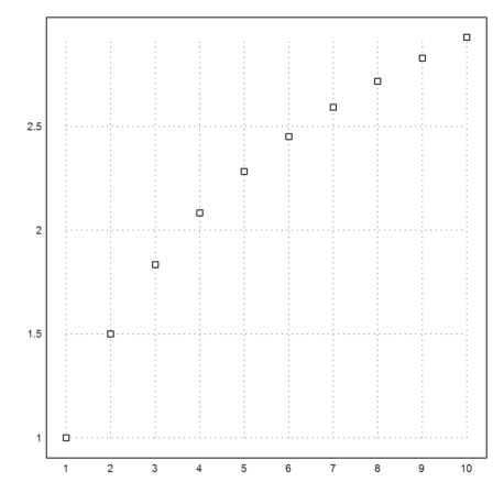
An interesting command is mxmtable(), which creates a table of values using Maxima. It prints the values and a plot of the values. The second argument is the variable name.
>mxmtable("sum(1/k,k,1,n)","n",1,10);
            1
          1.5
      1.83333
      2.08333
      2.28333
         2.45
      2.59286
      2.71786
      2.82897
      2.92897
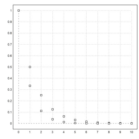
Even a table of two variables can be created.
>mxmtable(["2^-n","3^-n"],"n",0,10,print=0);
Note that all variables in Maxima are different from the variables in Euler. But symbolic expressions are known to both worlds. In Euler, they are strings, which print as a symbolic formula via Maxima.
>expr &= x/(1+x^2)
                                  x
                                ------
                                 2
                                x  + 1
For numerical values and small matrices, we can use &:= to set a value for Maxima and Euler. This value can be used in all symbolic expressions.
>v &:= 1:10; &v
[1, 2, 3, 4, 5, 6, 7, 8, 9, 10]
In Euler, it is just an ordinary numerical variable.
>v
[1, 2, 3, 4, 5, 6, 7, 8, 9, 10]
Note that changing the variable in Euler does not change the value in Maxima.
>v[4]=10
[1, 2, 3, 10, 5, 6, 7, 8, 9, 10]
>&v
[1, 2, 3, 4, 5, 6, 7, 8, 9, 10]
If you need to change both variables, you need to set the Maxima value once more.
>v[4]=10; v &:= v; &v
[1, 2, 3, 10, 5, 6, 7, 8, 9, 10]
This is a consequence of the two worlds, Euler and Maxima. Usually, you will not want to compute in both worlds simultaneously.
For very large matrices, use mxmset(). Sending v in a string will not work.
>mxmset("v",1:1000); &v[1000]
1000
Note, that setting the value in Maxima and Euler all the time is not a good idea in functions. The transfer and the processing in Maxima will slow down your function considerably.
If you need to use Maxima in Euler functions, reduce the transfer to the absolute minimum. It might be a good idea to define a Maxima function if that is possible.
Symbolic algebra is useful to help numerical algorithms in Euler. We can use the Newton method, and let Maxima compute the derivative of the function for us.
>longestformat; newton("x^x-2",&diff(x^x-2,x),2)
1.559610469462369
The utility function "mxmnewton" makes this easier.
>mxmnewton("x^x-2",2)
1.559610469462369
To check, we use the bisection method.
>bisect("x^x-2",1,2)
1.559610469462314
The interval Newton method provides a guaranteed inclusion of the solution. Note that the bisection does not have this accuracy.
>mxminewton("x^x-2",~1,2~)
~1.559610469462368,1.559610469462371~
Maxima can also be used for the Newton method in several dimensions.
The utility function "mxmnewtonfxy" uses the Newton method to find a point where both expressions are 0.
>longformat; mxmnewtonfxy("x^2+y^2-10","x+y-4",[1,2])
[1, 3]
Let me demonstrate how to do this without utility functions.
First you define the function as a symbolic expression.
>fexpr &= [x^2+y^2-10,x+y-4]
                        2    2
                      [y  + x  - 10, y + x - 4]
Then you define the function, using the vector syntax for the function arguments. In general, you need a function, which takes a vector and returns a vector. We define it as a symbolic function.
>function f([x,y]) &= fexpr
                        2    2
                      [y  + x  - 10, y + x - 4]
Moreover, you need a function, which takes a vector, and returns the Jacobian. To compute the derivatives, use Maxima at compile time.
>function Df([x,y]) &= jacobian(fexpr,[x,y])
                             [ 2 x  2 y ]
                             [          ]
                             [  1    1  ]
Indeed, the function is defined as expected.
>type Df
function Df ([x, y])
useglobal; return matrix([2*x,2*y],[1,1])
endfunction
Now you can start the Newton method.
>newton2("f","Df",[1,4])
[1, 3]
Or you can start an interval Newton method, which provides a guaranteed inclusion.
>inewton2("f","Df",[1,4])
[ ~0.999999999999998,1.000000000000003~,
~2.999999999999997,3.000000000000003~ ]
Sometimes, Maxima is asking questions. If this happens, enter the answer in the next input line.
>:: integrate(x^n,x)
Is n equal to - 1?
Here, we choose nonzero.
>:: nonzero
Acceptable answers are yes, y, Y, no, n, N.
Is n equal to - 1?
In symbolic expressions, many questions will be answered automatically. By default the user gets a message.
>&integrate(x^n,x)
Answering "Is n equal to - 1?" with "no"

                                n + 1
To avoid questions, you can make assumptions.
>&assume(n>0); &integrate(x^n,x), &forget(n);
                                 n + 1
                                x
                                ------
                                n + 1
Let us generate a matrix in Euler and Maxima.
>A:=2*id(3); A:=setdiag(A,-1,1); A&:=setdiag(A,1,1); short A
          2           1           0
          1           2           1
          0           1           2
Compute the eigenvalues in Maxima.
>ev &= eigenvalues(A)
[[2 - sqrt(2), sqrt(2) + 2, 2], [1, 1, 1]]
This returns a vector with two elements, the eigenvalues and their multiplicities. We extract and evaluate the eigenvalues. Remember that &:... evaluates a symbolic expression.
>&:ev[1]
[0.585786437627, 3.41421356237, 2]
This is the same result as numerically in Euler.
>re(eigenvalues(A))
[0.585786437627, 2, 3.41421356237]
Here is an integral, where Maxima uses the function erf for the result.
>&integrate(exp(-x^2/2),x,-1,1)
                                            1
                    sqrt(2) sqrt(pi) erf(-------)
                                         sqrt(2)
We can evaluate the last expression numerically.
>&integrate(exp(-x^2/2),x,-1,1); longest(%())
1.711248783784298
This can be done in one step.
>longest &:integrate(exp(-x^2/2),x,-1,1)
1.711248783784298
We can also check with the Romberg method integrating the Gauß distribution.
>longest romberg("exp(-x^2/2)",-1,1)
1.71124878378431
The line integral of the Gauß normal distribution is exactly known to Maxima, of course.
>&integrate(exp(-x^2/2),x,minf,inf)/sqrt(2*pi)
1
For an example, we compute the partial fraction decomposition of
![]()
It is easy to get the partial fraction decomposition in Maxima automatically.
>&partfrac((x-1)/(x^2*(x+1)),x)
                               2     2   1
                           - ----- + - - --
                             x + 1   x    2
                                         x
Let us try to do that by hand.
>&remvalue(A,B,C); &ratsimp(A/x+B/x^2+C/(x+1)), enum &= expand(num(%))
                     2                   2
                    x  C + (x + 1) B + (x  + x) A
                    -----------------------------
                                3    2
                               x  + x


                      2                2
                     x  C + x B + B + x  A + x A
Now we compare coefficients and solve for A, B and C.
>sol &= solve([coeff(enum,x,0)=-1,coeff(enum,x,1)=1,coeff(enum,x,2)=0])
[[C = - 2, A = 2, B = - 1]]
Then substitute the solutions back.
>&A/x+B/x^2+C/(x+1) with sol[1]
                               2     2   1
                           - ----- + - - --
                             x + 1   x    2
                                         x
For another example, here is a curve in the form of an "8".
>plot2d("sin(x)","sin(x)*cos(x)",xmin=-pi,xmax=pi,r=1):
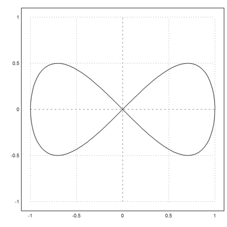
We compute the curve differential using Maxima.
>ds &= trigsimp(sqrt(diff(sin(x),x)^2+diff(sin(x)*cos(x),x)^2))
                             4           2
                   sqrt(4 cos (x) - 3 cos (x) + 1)
Now we can compute the length of the curve numerically with Euler.
>longest romberg(ds,-pi,pi)
6.097223470105731
Maxima for Euler can load packages.
>&batch(solve_rec);
We solve the Fibonacci recursion numerically.
>sol &= solve_rec(h[n+2]=h[n+1]+h[n],h[n])
                           n          n                n
              (sqrt(5) - 1)  %k  (- 1)    (sqrt(5) + 1)  %k
                               1                           2
         h  = ------------------------- + ------------------
          n               n                        n
                         2                        2
To get h1=1, h2=1, we solve for the constants.
>&solve([subst(0,n,rhs(sol))=0,subst(1,n,rhs(sol))=1],[%k[1],%k[2]])
                               1              1
                  [[%k  = - -------, %k  = -------]]
                      1     sqrt(5)    2   sqrt(5)
And substitute the constant back to the solution. The right hand side is our desired formula.
>&sol with %[1]; sol &= rhs(%); $sol
![]()
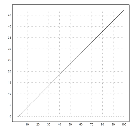
Now we can plot the logarithmic growth of the Fibonacci numbers.
>n:=1:100; m:=sol(n); mxmeval("sol",n:=1:100); plot2d(n,log(m)):
The following limit is no problem.
>sx &= (1+1/x)^x, &limit((1+1/x)^x,x,inf)
                                1     x
                               (- + 1)
                                x


                                  E
If we want to estimate the convergence, we need to use Taylor series methods. Maxima does that automatically.
>&limit(x*(sx-E),x,inf)
                                   E
                                 - -
                                   2
Even finer:
>&tlimit(x*(x*(sx-E)+E/2),x,inf)
                                 11 E
                                 ----
                                  24
Let us interpolate with a rational function.
>p &= (a*x+b)/(1+c*x)
                               a x + b
                               -------
                               c x + 1
To find a,b,c, we use the solve command of Maxima.
>sol &= solve([(p with x=0)=1,(p with x=1)=-1,(p with x=2)=2],[a,b,c])
                             7               5
                     [[a = - -, b = 1, c = - -]]
                             6               6
Substitute back into p.
>fres &= ratsimp(p with sol[1])
                               7 x - 6
                               -------
                               5 x - 6
We can also make a symbolic function out of this.
>function f(x) &= fres
                               7 x - 6
                               -------
                               5 x - 6
Test the interpolation values.
>longformat; f([0,1,2])
[1, -1, 2]
It is possible to output a symbolic term with Latex, if you have Latex installed. However this will slow down the execution of your notebooks.
It might be better to use "maxima: formula" in a comment. Here is an example.
![]()
The code for this was
maxima: 'integrate(x^2*log(x),x)=factor(integrate(x^2*log(x),x))+c
Here is a direct output of a symbolic expression in the usual Euler output.
>$factor(diff(x^4*exp(-x^2),x))
![]()
If you want to demonstrate a computation, the easiest way is the following.
>&showev('integrate(x^3*exp(x^2),x))
                                               2
                      /      2        2       x
                      [  3  x       (x  - 1) E
                      I x  E   dx = ------------
                      ]                  2
                      /
The ' prevents the evaluation of a function. You can use this in Maxima comments too.
![]()
Printing of an expression simplifies it. Therefore, the following does only work in direct input.
>:: factor(323247)
3 19 53 107
If you want to do this with symbolic expression, you need to store the result to a variable, which you print un-evaluated.
>h&=factor(323247); &'h
3 19 53 107
To get the Latex code of an expression, use tex(...).
>&eigenvalues([1,2;3,4])[1], tex(%)
                      5 - sqrt(33)  sqrt(33) + 5
                     [------------, ------------]
                           2             2

\left[ \frac{5-\sqrt{33}}{2} , \frac{\sqrt{33}+5}{2} \right]
Here is the direct output.
>$eigenvalues([1,2;3,4])[1]
![]()
Gnuplot is set in EMT so that it exports a graphics file in PNG format. The file can be found in your home directory. On my system, it is the following file.
>eulerhome()+"gnuout.png"
C:\Users\Rene\Euler\gnuout.png
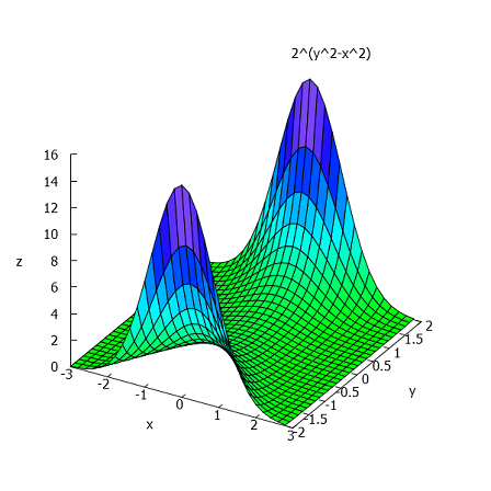
The result of the plots can be imported into EMT with a colon after the symbolic command or with the function mxmins().
>&plot3d(2^(y^2-x^2),[x, -3, 3],[y, -2, 2]):
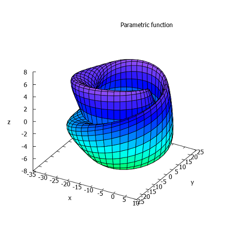
>expr1 &= 5*cos(x)*(cos(x/2)*cos(y)+sin(x/2)*sin(2*y)+3)-10; ...
 expr2 &= -5*sin(x)*(cos(x/2)*cos(y)+sin(x/2)*sin(2*y)+3); ...
 expr3 &= 5*(-sin(x/2)*cos(y) + cos(x/2)*sin(2*y)); ...
 &plot3d([expr1,expr2,expr3],[x,-pi,pi],[y,-pi,pi],[grid, 40, 40]):
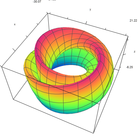
Here is a plot of the same surface with plot3d() of EMT.
>plot3d(expr1,expr2,expr3,r=pi,>spectral, ...
   scale=[1,1,2],n=200,grid=20,height=50°,zoom=3.2):
To change the aspect ratio of a plot you need to call mxmpng().
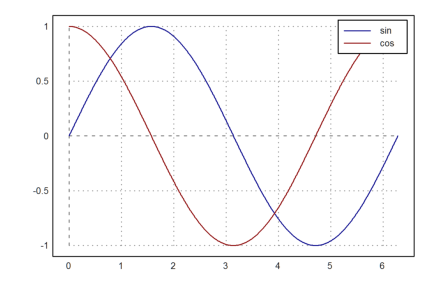
>mxmsetpng(600,400); ...
 &plot2d([sin(x),cos(x)],[x,0,2*pi]):
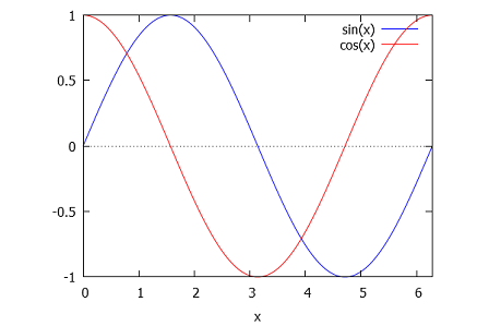
Again, here is the same plot in EMT.
>aspect(3/2); ...
 plot2d(["sin(x)","cos(x)"],0,2pi,color=[blue,red]); ...
 labelbox(["sin","cos"],colors=[blue,red]):
You should reset everything to the default values for further plots in the same notebook.
>reset(); mxmsetpng();
Maxima runs parallel to Euler. By default, it is started, when Euler starts. It is stopped and restarted, when Euler restarts or loads a new notebook.
The programs communicate via pipes. Elements are transported in text form. The speed issue is usually not important, since the symbolic computations take a lot of time anyway. To keep things fast, you need to do them numerically in Euler.
Both worlds are separated. They have separate variables and functions. Symbolic variables and functions are just a way to define and handle items in both worlds.
So the following symbolic variable is known to Euler and Maxima.
>a &= x^5;
In Maxima this expression is stored in the variable a.
>:: a
                                   5
                                  x
In Euler, it is stored in the variable a too, but as a string.
>""+a
x^5
The variable has the flag "symbolic", and will print as a symbolic variable. The print is done by Maxima using the value stored in the Euler string.
>a
                                   5
                                  x
Symbolic expressions are strings in Euler. If a value is needed both in Euler and Maxima, use &:=.
>M &:= [1,2;3,4];
This is a matrix value in Maxima. Note that the symbolic expression replaced the matrix syntax with the proper matrix() command in Maxima.
>:: M
                               [ 1  2 ]
                               [      ]
                               [ 3  4 ]
The matrix has integer elements, since it was defined with integer values.
>:: eigenvalues(M)
                   sqrt(33) - 5  sqrt(33) + 5
               [[- ------------, ------------], [1, 1]]
                        2             2
In Euler, this is just a numerical matrix.
>eigenvalues(M)
[ -0.372281+0i , 5.37228+0i ]
The assignment &:= converts values to fractions for Maxima. The reason is that the value of Maxima should be a symbolic translation of the value of Euler.
>a &:= pi; &a
                               1146408
                               -------
                               364913
If you do not like this, use mxmset().
>mxmset("a",pi); &a
3.141592653589793
A symbolic function is defined as a numerical function in Euler and as a symbolic function in Maxima at the same time. You saw a lot of examples on this page.
But there are also purely symbolic functions. These functions are defined only in Maxima. The body of the function is not evaluated at compile time.
>function D2(g,x) &&= diff(g,x,2)
diff(g, x, 2)
A symbolic function would not work, since diff(g,x,2) evaluates to 0. It helps to think of D2 as a macro, which takes the second derivative of g at run time.
>&D2(x^4,x)
                                    2
                                12 x
There are also purely symbolic values, which do not mess with Euler values.
>a &&= x+1
x+1
>a
3.14159265359
It is possible to call Maxima at compile time in longer Euler functions, just as in one-line functions.
>function f(x) ...
 return &:"diff(x^x,x)"
 endfunction
>type f
function f (x)
return x^x*(log(x)+1)
endfunction
You can learn more details on this in the tutorial about programming.
Symbolic expressions are scanned by EMT before they go to Maxima. E.g., the | is replaced by a comma to allow flags. If you do not want this you need to escape with \|.
The following defines an infix operator | in Maxima (same as multiplication). Since := is replaced by :, we need to use \:=.
>:: infix("\|",115); a\|b \:= a*b
a | b := a b
It might be easier to use the direct mode if you want to delve into the Maxima syntax.
>::: infix("|",115)$ a|b := a*b
a | b := a b
Now we can use the new operator. But we must either escape it with \|, or start the complete symbolic expression with ! (prevents replacements).
>&!5|4
20
Another replacement is @var for a numerical variable.
>a=67; &2*@a
134
Here is a block command of Maxima with the more natural := syntax. You can just as well use :.
>&block([x], for i:=1 thru 3 do x:=1+1/x, x)
                                1
                            --------- + 1
                              1
                            ----- + 1
                            1
                            - + 1
                            x
The definition of functions works with := because the replacement recognizes this.
>:: f(x) := x^3
                                       3
                              f(x) := x
>&f(5)
125