Historical stock data are available for free from
If you open this link, you see the Google data from 2013. On the bottom of the page, you see a link to download the CVS (comman separated values) file with the data. It is in English format, so you cannot open it with Excel on German systems, but you can import it anyway.
The following function is an example that shows how to read data from a CSV file. We skip the heading and interpret only the 7th column. The data are in reverse order.
>function readcsv (filename) ...
 open(filename+".csv","r");
 getline();
 D=[];
 repeat;
    line=getline();
    until strlen(line)==0;
    s=strtokens(line,",");
    D=D|evaluate(s[7]);
 end;
 close();
 return fliplr(D);
 endfunction
Let us read the three stocks.
>SI=readcsv("SI"); ...
 IBM=readcsv("IBM"); ...
 Google=readcsv("Google");
The following shows the data.
>Data=[SI;IBM;Google]; ...
 col=[green,blue,red]; names=["Siemens","IBM","Google"]; ...
 plot2d(Data,color=col,title="Price Development"); ...
 labelbox(names,colors=col,>left,x=0.1,y=0.5,w=0.3):
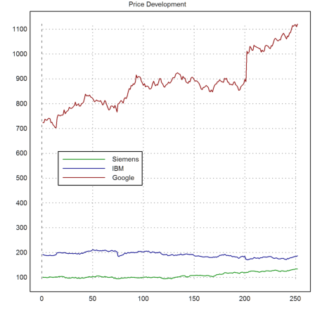
Next we like to print the development of these stocks. We adjust the stock values (in rows of the matrix "data") so that each begins with 1, and use the corporate colors to plot the curves.
>NormedData=Data/Data[:,1]; ...
 plot2d(100*NormedData,color=col,title="Portfolio Development",yl="%");  ...
 labelbox(names,colors=col,>left,x=0.1,w=0.3):
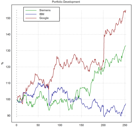
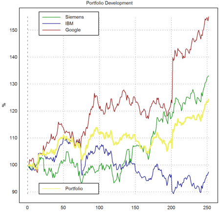
As an example, we add the development of a portfolio with 55, 144, 34 assets of each stock.
>c=[55,155,34]; V=c.Data; ...
 plot2d(100*V/V[1],color=yellow,thickness=3,>add); ...
 labelbox("Portfolio",colors=yellow,x=0.1,y=0.9,w=0.3,>left):
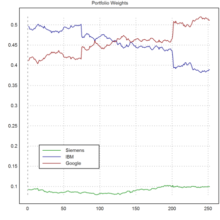
The following shows the weights of each stock in our portfolio.
>P=c'*Data; W=P/V; ...
 plot2d(W,color=col,title="Portfolio Weights"); ...
 labelbox(names,colors=col,>left,x=0.1,y=0.7,w=0.3):
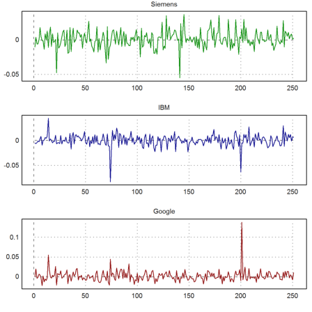
Here is another plot, which shows the daily returns.
>m=cols(P); PR=differences(P)/head(P,-2); ...
 figure(3,1);  ...
 for i=1:3; figure(i); plot2d(PR[i],title=names[i],color=col[i]); end; ...
 figure(0):
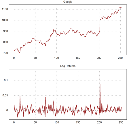
Often the log returns are used. Let us combine a stock and its log returns.
>figure(2,1); ...
 figure(1); plot2d(Google,title="Google",color=red);  ...
 figure(2);  ...
   plot2d(differences(log(Google)),color=red,title="Log Returns");  ...
 figure(0):
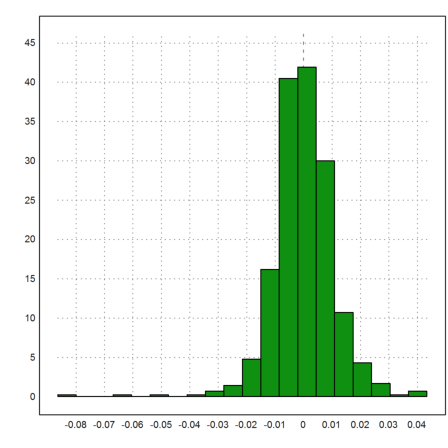
The distribution of the log returns is disturbed by one jump.
>d=differences(log(Google)); plot2d(d,distribution=20):
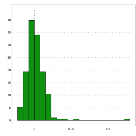
Besides that it looks almost normal distributed. Of course, the one outlier can spoil all statistical analysis or predictions.
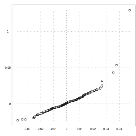
To compare this distribution with the normal distribution, we use a quantile-quantile plot of our data and random data.
>dm=mean(d); dv=dev(d); data=normal(size(d))*dv+dm; ...
 plot2d(sort(data),sort(d),>points):
You can also open the URL to the CVS file directly and read the data from it.
>function getstock(stock,date1,date2) ...
 s="https://ichart.finance.yahoo.com/table.csv?s="+stock;
 {y,m,d}=date(date1); s=s+''&a=''+(m-1)+''&b=''+d+''&c=''+y;
 {y,m,d}=date(date2); s=s+''&d=''+(m-1)+''&e=''+d+''&f=''+y;
 s=s+''&g=d&ignore=.csv'';
 v=[];
 urlopen(s);
 heading=strtokens(urlgetline(),",");
 repeat
    line=urlgetline();
    line=strtokens(line,",");
    if length(line)<2 then break; endif;
    date=day(line[1]);
    for k=2:cols(line);
        date=date|line[k]();
    end;
    v=v_date;
    until urleof();
 end;
 urlclose();
 return {v,heading};
 endfunction
Now we can read the data directly from the web page.
>{v,hd}=getstock("GOOG",day(2013,1,1),day(2014,12,31));
Let us print the three most important columns with writetable().
>i=[1,3,4,7];  ...
 writetable(v[1:min(rows(v),20),i],labc=hd[i],date=[1],wc=[12,10,10,12]);
        Date      High       Low   Adj Close
  2014-12-31     532.6     525.8       526.4
  2014-12-30    531.15    527.13      530.42
  2014-12-29    535.48    530.01      530.33
  2014-12-26    534.25    527.31      534.03
  2014-12-24    531.76    527.02      528.77
  2014-12-23    534.56    526.29      530.59
  2014-12-22    526.46    516.08      524.87
  2014-12-19    517.72    506.91      516.35
  2014-12-18    513.87     504.7       511.1
  2014-12-17       507    496.81      504.89
  2014-12-16    513.05       489      495.39
  2014-12-15     523.1    513.27       513.8
  2014-12-12     528.5    518.66      518.66
  2014-12-11    533.92     527.1      528.34
  2014-12-10    536.33    525.56      526.06
  2014-12-09    534.19     520.5      533.37
  2014-12-08       531    523.79      526.98
  2014-12-05    532.89    524.28      525.26
  2014-12-04    537.34    528.59      537.31
  2014-12-03       536    529.26      531.32
The following functions makes it easy to get the values of a specific asset from some time in the past till now.
>function plotsince (stock,year,logreturns=false) ...
 {v,hd}=getstock(stock,day(year,1,1),daynow());
 dates=fliplr(v[,1]'); dates=dates; values=fliplr(v[,7]');
 years=(dates-dates[1])/365.25+year;
 if logreturns then
    figure(2,1);
    figure(1); plot2d(years,values);
    figure(2); plot2d(head(years,-2),differences(log(values)));
    figure(0);
 else
    plot2d(years,values);
 endif;
 settitle(stock);
 endfunction
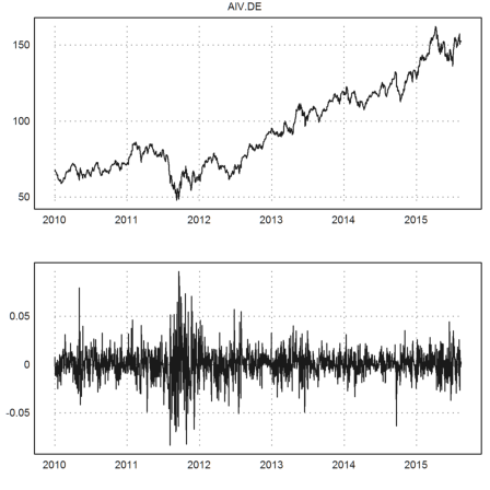
We load the German Allianz data since 2010. The plot also shows the daily log returns.
>plotsince("AlV.DE",2010,true):
There is a utility file for this.
>load getstock;
It works a bit differently. With two dates it reads the data between the dates. With one date, it reads the data till now.
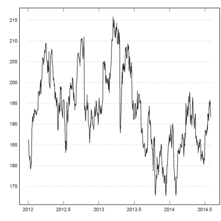
>v=getstock("IBM",day(2012,1,1));
The file contains the following routine to plot the data.
>showstock(v):
The matrix v is a nx2 matrix with dates in the first and values in the second column. Let us extract the values and the logarithmic returns of the data.
>d=v'[2]; r=differences(log(d)); plot2d(r,>distribution):
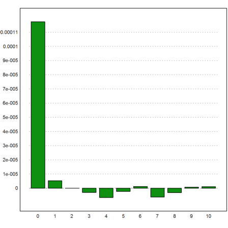
We can also compute correlations between returns at day n and day n+k.
![]()
For k=0, we get the variance, assuming that the mean return is 0.
>rm=r-mean(r); ...
 c=[]; for k=0 to 10; c=c|mean(head(rm,-k-1)*tail(rm,k+1)); end;
Indeed the returns of successive days do not show much correlation.
>columnsplot(c,lab=0:10):