The aim of this example is to show how tables can from R can be used in EMT. EMT cannot cope with R in terms of statistical functions. But often it is nice to work with data in EMT. As you will see, many statistical functions are available or can be programmed in EMT.
Often, doing things without a specific statistical software provides more insight than using a black box.
The data used for this notebook are form "A Handbook of Statistical Analysis using R" by Everitt and Hothorn.
The file "forbes2000.cvs" was imported in R and exported to a comma separated file with the following commands.
  >install.packages("HSAUR")
  >library("HSAUR")
  >write.table(Forbes2000,
    file="\\users\\rene\\desktop\\forbes2000.csv",
    sep=",",quote=FALSE)
Here are the first 6 lines of this file.
>printfile("forbes2000.csv",5)
rank,name,country,category,sales,profits,assets,marketvalue
1,1,Citigroup,United States,Banking,94.71,17.85,1264.03,255.3
2,2,General Electric,United States,Conglomerates,134.19,15.59,626.93,328.54
3,3,American Intl Group,United States,Insurance,76.66,6.46,647.66,194.87
4,4,ExxonMobil,United States,Oil & gas operations,222.88,20.96,166.99,277.02
Obviously, there is heading for the table, and a heading for each row of data.
The file can be imported to EMT with readtable(). The columns 2,3,4 contain tokes, which are connected in a string vector "toks". The file uses the string "NA" for "not available".
>{table,head,toks}=readtable("forbes2000.csv", ...
   >rlabs,ctok=[2,3,4],separator=",",NA="NA");
As you see the tokens have been translated to numbers, which are indices in the vector "toks".
>table
Real 2000 x 8 matrix

            1             1             2             3     ...
            2             4             2             5     ...
            3             6             2             7     ...
            4             8             2             9     ...
            5            10            11             9     ...
            6            12             2             3     ...
            7            13            11             3     ...
            8            14            15            16     ...
            9            17             2            18     ...
           10            19             2            20     ...
           11            21            22            18     ...
           12            23            24            18     ...
           13            25            26             9     ...
           14            27             2             7     ...
           15            28             2             3     ...
           16            29             2            30     ...
           17            31            32             9     ...
           18            33            32             3     ...
           19            34            11             3     ...
           20            35             2            18     ...
    ...
There are 2000 entries in the table.
>size(table)
[2000, 8]
The header strings are the following.
>head
rank
name
country
category
sales
profits
assets
marketvalue
We define a function which finds the column number by the name of the column.
>function c(s) := indexof(head,s);
We can now extract a column from the table. For a try, we compute the mean and the median of the sales.
>sales=tablecol(table,c("sales")); mean(sales), median(sales)
9.69701
4.365
Here is the logarithmic distribution of the sales.
>plot2d(logbase(sales,10),>distribution):
What categories are there?
>category=tablecol(table,c("category"))
[3,  5,  7,  9,  9,  3,  3,  16,  18,  20,  18,  18,  9,  7,  3,  30,
9,  3,  3,  18,  16,  39,  9,  42,  3,  45,  3,  18,  16,  45,  51,
39,  45,  18,  5,  3,  9,  9,  3,  18,  3,  65,  30,  68,  71,  42,
3,  3,  16,  18,  16,  3,  7,  3,  9,  18,  3,  71,  7,  20,  65,  7,
42,  42,  93,  39,  3,  3,  98,  65,  16,  93,  7,  16,  16,  5,  3,
42,  3,  42,  9,  16,  30,  45,  65,  3,  9,  123,  30,  3,  93,  3,
45,  98,  5,  18,  133,  7,  3,  16,  20,  39,  18,  39,  7,  3,  145,
42,  9,  65,  133,  45,  30,  16,  93,  45,  9,  42,  42,  123,  42,
164,  133,  7,  18,  3,  9,  3,  42,  3,  30,  133,  3,  179,  145,
3,  164,  185,  7,  188,  7,  191,  98,  5,  196,  3,  164,  3,  3,
20,  3,  93,  98,  3,  39,  208,  93,  18,  7,  3,  18,  145,  5,  45,
42,  196,  20,  5,  145,  7,  93,  20,  93,  188,  45,  196,  7,  93,
3,  16,  42,  93,  123,  9,  3,  68,  45,  164,  93,  18,  93,  98,
45,  7,  3,  179,  20,  196,  93,  3,  39,  45,  7,  68,  185,  164,
45,  65,  16,  7,  45,  3,  9,  9,  39,  51,  45,  123,  191,  5,  3,
18,  3,  20,  208,  42,  7,  93,  18,  3,  98,  98,  71,  39,  179,
45,  39,  51,  3,  196,  145,  7,  9,  191,  93,  39,  3,  196,  123,
68,  3,  39,  3,  185,  185,  93,  7,  93,  188,  3,  39,  3,  3,  9,
9,  123,  196,  3,  93,  98,  7,  164,  9,  65,  164,  39,  7,  42,
196,  20,  93,  9,  145,  164,  93,  133,  16,  18,  9,  123,  45,
 ... ]
This is a vector of numbers. To translate back to strings wih use the numbers as indices in the vector "toks".
>unique(toks[category])
Aerospace & defense
Banking
Business services & supplies
Capital goods
Chemicals
Conglomerates
Construction
Consumer durables
Diversified financials
Drugs & biotechnology
Food drink & tobacco
Food markets
Health care equipment & services
Hotels restaurants & leisure
Household & personal products
Insurance
Materials
Media
Oil & gas operations
Retailing
Semiconductors
Software & services
Technology hardware & equipment
Telecommunications services
Trading companies
Transportation
Utilities
Only in column 6 (profits) are some entries not available.
>mnonzeros(isNAN(table))
          772             6
         1085             6
         1091             6
         1425             6
         1909             6
The function tablecol() would skip these items. But for statistical purposes, we would like to reduce the table to available items only. So we throw out these lines.
>ivalid=nonzeros(!isNAN(table[,6]));
We make a function, which extracts a column from the table reducing to the lines which have only available data.
>function d(s) := table[ivalid,c(s)]';
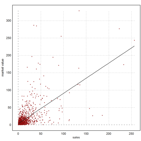
Let us plot the relation between sales and market value.
>plot2d(d("sales"),d("marketvalue"), ...
   >points,color=red,style="..",xl="sales",yl="market value");
There seem to be some yet unprofitable items. However, a regression seems to work quite well.
>p=polyfit(d("sales"),d("marketvalue"),1); ...
 plot2d("polyval(p,x)",>add):
Which company has the least or highest profit/sales ratio?
>rat=d("profits")/d("sales"); ex=extrema(rat)
[-2.80198, 1493, 26, 1956]
The elements ex[2] and ex[4] are the indices of the minimum and the maximum. To find the company, we need the vector of companies, and we have to look the index up in the vector of string tokens.
>d("name")[ex[[2,4]]], toks[%]
[1580,  2049]
Eurotunnel
Custodia Holding
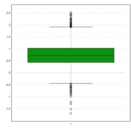
The logarithmic distribution of the market values can be indicated in the following box plot. It is not normally distributed.
>boxplot(logbase(d("marketvalue"),10)):
To print the table, we can use writetable(). In the following, we restrict to sales and profits, and print only the first 5 lines.
We need to translate the first column into strings.
>ci=[c("name"),c("sales"),c("profits")];  ...
 writetable(table[1:5,ci],ctok=[1],tok=toks, ...
   wc=[30,10,10],labc=head[ci],fixed=2)
                          name     sales   profits
                     Citigroup     94.71     17.85
              General Electric    134.19     15.59
           American Intl Group     76.66      6.46
                    ExxonMobil    222.88     20.96
                            BP    232.57     10.27
For the following, we reduce our table to the lines which have only available profits.
>vtable=table[ivalid];
Let us make a function which prints this for selected lines, but only for the companies with available profits.
>function writesp (i) ...
     useglobal;
     ci=[c("name"),c("sales"),c("profits")];  ...
     writetable(vtable[i,ci],ctok=[1],tok=toks, ...
        wc=[30,10,10],labc=head[ci],fixed=2);
 endfunction
To get the lines sorted by sales, we use the fact that sort() returns the indices of the sorted elements.
>{dummy,i}=sort(d("sales"));
Now we can print the 5 companies with the lowest and the highest sales.
>writesp(i[1:5])
                          name     sales   profits
              Custodia Holding      0.01      0.26
        Central European Media      0.11      0.31
              Minara Resources      0.17      0.34
                  Buenaventura      0.17      0.11
                 Denway Motors      0.19      0.14
>writesp(i[-(1:5)])
                          name     sales   profits
               Wal-Mart Stores    256.33      9.05
                            BP    232.57     10.27
                    ExxonMobil    222.88     20.96
                General Motors    185.52      3.82
                    Ford Motor    164.20      0.76
To print a specific company, we need to find its line in "vtable". Let us make a function fo this. It has to look up the number of the string item in "toks", then the index of the number in the company column.
>function icompany(s) := indexof(d("name"),indexof(toks,s));
As a benefit, the function will work for string vectors too.
>writesp(icompany(["Eurotunnel","Custodia Holding"]))
                          name     sales   profits
                    Eurotunnel      1.01     -2.83
              Custodia Holding      0.01      0.26
Data of two groups estimating the width of a room in feet and meters.
>printfile("roomwidth.csv",5)
unit,width
1,metres,8
2,metres,9
3,metres,10
4,metres,10
>{table,head,toks}=readtable("roomwidth.csv", ...
   >rlabs,ctok=[1],separator=",",NA="NA");
There are only two tokens, metres and feet.
>toks
metres
feet
With the following commands we extract the estimates in meters and feet from the data. The data in feet are converted to meters.
>u=tablecol(table,1); w=tablecol(table,2); ...
 imeters=nonzeros(u==1); ifeet=nonzeros(u==2); ...
 wfeet=w[ifeet]*feet$; wmeters=w[imeters];
Let us compare the two rows of data.
>quartiles(wmeters), quartiles(wfeet)
[8,  11,  15,  17,  25]
[7.3152,  10.8204,  12.8016,  14.6304,  19.2024]
We can also produce box plots side by side.
>figure(1,2);  ...
 figure(1); boxplot(wmeters,lab="meters",range=[0,50]);  ...
 figure(2); boxplot(wfeet,lab="feet",range=[0,50]);  ...
 figure(0):
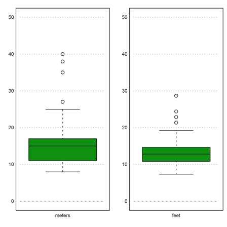
It seems that the estimates in meters are higher. Indeed, the rank test says that the estimates are higher with alpha=1.5%.
>ranktest(wmeters,wfeet)
0.0140344278866
The statistics for the Mann-Whitney-U-Test is usually computed via sums of ranks.
However, it can also be computed by counting the number of pairs M>F where M is an estimate in meters and F an estimate in feet. In EMT, this is very easy to get.
>U=totalsum(wmeters>wfeet')
1891
For equal distributions, The expected number is n*m/2. The correct statistics of U is approximately normally distributed as
![]()
We see that our U is 2.2 standard deviations higher than the expected value.
>m=cols(wmeters); n=cols(wfeet); m*n/2, (U-%)/sqrt(n*m*(n+m+1)/12)
1518
2.19632267635
This is precisely the alpha-value of our rank test.
>1-normaldis(U,m*n/2,sqrt(n*m*(n+m+1)/12))
0.0140344278866
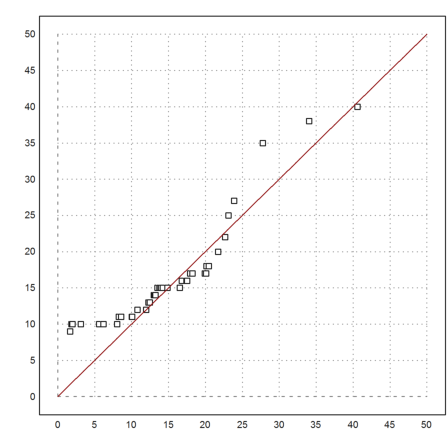
The Q-Q-plot shows that the estimates in meters have too many high outliers compared to the normal distribution. For this plot, we generate a sample of the same size and compare the two sorted samples point by point.
>x=randnormal(1,cols(wmeters),mean(wmeters),dev(wmeters)); ...
 plot2d(sort(x),sort(wmeters),>points,a=0,b=50,c=0,d=50); ...
 plot2d("x",color=red,>add):
The aim is to demonstrate density estimators.
The data contain the length of an eruption and the waiting time for the next eruption of the Old Faithful geyser.
>printfile("faithful.csv",5)
eruptions,waiting
1,3.6,79
2,1.8,54
3,3.333,74
4,2.283,62
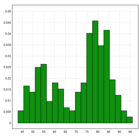
We read the table as usual and print a histogram of the waiting times.
>{table,head}=readtable("faithful.csv",>rlabs,separator=","); ...
 w=tablecol(table,2); plot2d(w,>distribution):
To smoothen out the histogram and get a density function, we fold the date with the Gauss kernel.
>function map ws (x;data=w,sigma=2) ...
   return sum(qnormal((data-x)/sigma))/(cols(data)*sigma)
 endfunction
>plot2d(w,>distribution,a=30,b=110,c=0,d=0.05,style="O",xl="min"); ...
 plot2d("ws",color=red,thickness=2,>add):
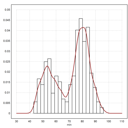
This looks like a sum of two distributions. One way to find the two different sets of data is clustering.
>load clustering; i=kmeanscluster(w',2);
We find 100 and 172 objects in each class.
>i1=nonzeros(i==1); n1=cols(i1), i2=nonzeros(i==2); n2=cols(i2), n=n1+n2;
100
172
Now we plot the two smoothed out densities.
>t=30:110;  ...
 plot2d(t,ws(t,w[i1])*n1/n,a=30,b=110,c=0,d=0.05,color=red); ...
 plot2d(t,ws(t,w[i2])*n2/n,>add,color=blue):
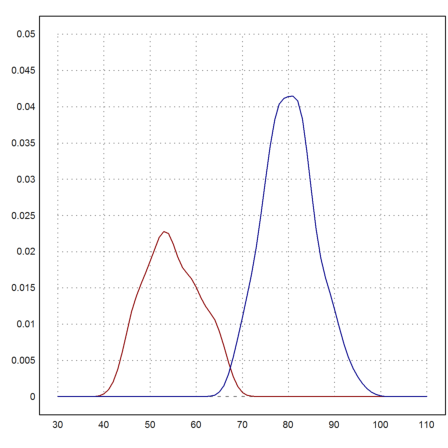
>mean(w[i1]), mean(w[i2])
54.75
80.2848837209
There is a clear connection between the length of the eruption and the waiting time for the next eruption.
>er=tablecol(table,1); plot2d(w,er,>points);  ...
 plot2d(w[i1],er[i1],>points,color=red,style="[]#",>add); ...
 plot2d(w[i2],er[i2],>points,color=blue,style="[]#",>add); ...
 p=polyfit(w,er,1); plot2d("polyval(p,x)",>add):