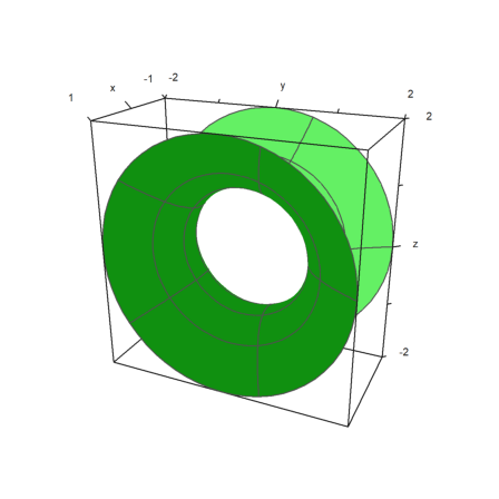
This is an introduction to 3D plots in Euler.
In general, Euler uses a central projection. By default, the view is from the positive x-y quadrant towards the origin x=y=z=0. Euler can plot
In all 3D plots Euler can produce red/cyan anaglyphs.
For the graph of a function, use
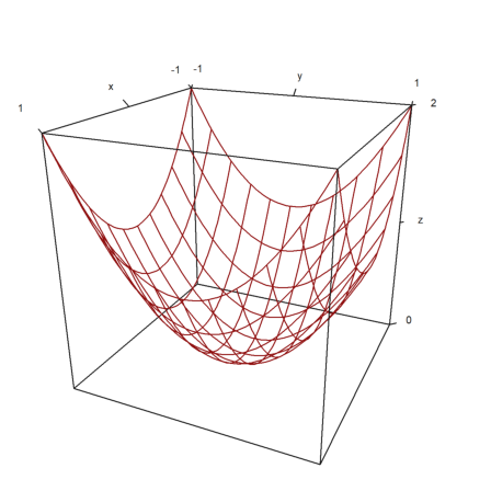
The default is a filled wire grid with different colors on both sides. Note that the default number of grid intervals is 10, but the plot uses the default number of 40x40 rectangles to construct the surface. This can be changed.
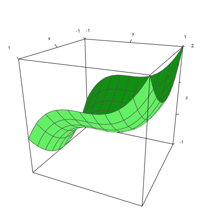
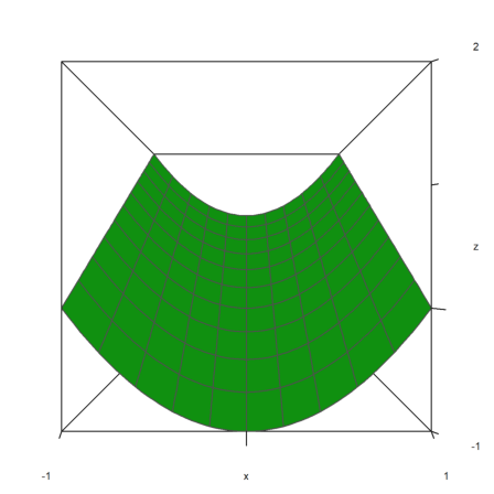
We use the default n=40 and grid=10.
>plot3d("x^2+y^2"):
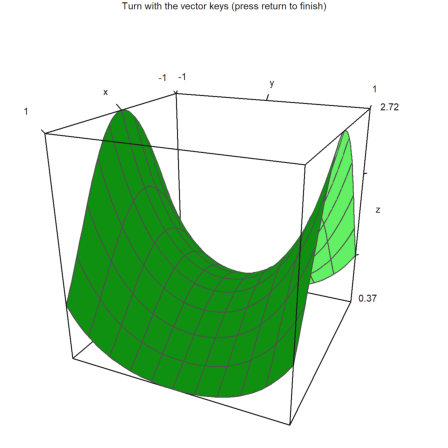
User interaction is possible with the >user parameter. The user can press the following keys.
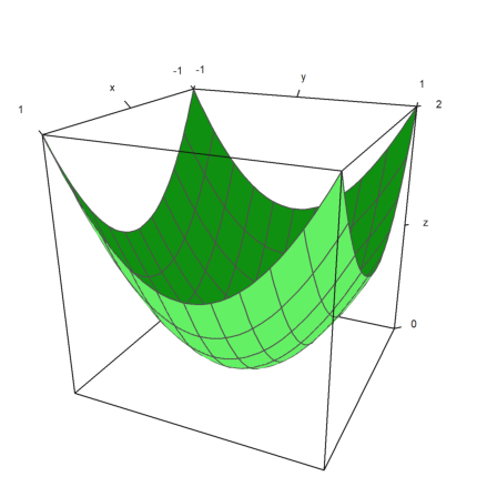
>plot3d("exp(-x^2+y^2)",>user, ...
   title="Turn with the vector keys (press return to finish)"):
The plot range for functions can be specified with
There are some parameters to scale the function or change the look of the graph.
fscale: scales to function values (default is <fscale).
scale: number or 1x2 vector to scale into x- and y-direction.
frame: type of frame (default 1).
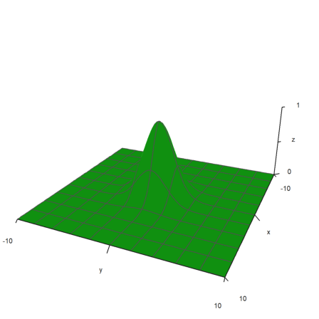
>plot3d("exp(-(x^2+y^2)/5)",r=10,n=80,fscale=4,scale=1.2,frame=3):
The view can be changed in many different ways.
The default values can be inspected or changed with the function view(). It returns the parameters in the order above.
>view
[5, 2.6, 2, 0.4]
A closer distance needs less zoom. The effect is more like a wide angle lens.
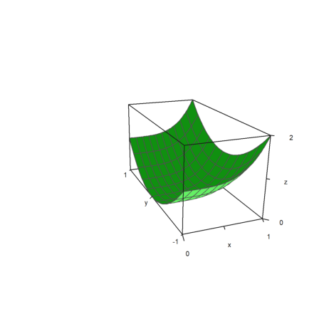
In the following example, angle=0 and height=0 look from the negative y-axis. The axis labels for y are hidden in this case.
>plot3d("x^2+y",distance=3,zoom=1.5,angle=0,height=0):
The plot looks always to the center of the plot cube. You can move the center with the center parameter.
>plot3d("x^4+y^2",a=0,b=1,c=-1,d=1,angle=-20°,height=20°, ...
   center=[0.4,0,0],zoom=2.5):
The plot is scaled to fit into a unit cube for viewing. So there is no need to change the distance or zoom depending on the size of the plot. The labels refer to the actual size, however.
If you turn this off with scale=false, you need to take care, that the plot still fits into the plotting window, by changing the viewing distance or zoom, and moving the center.
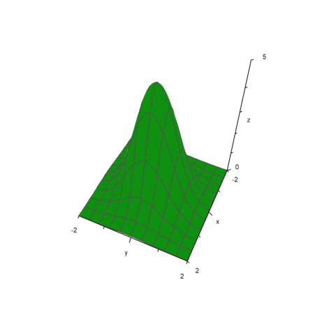
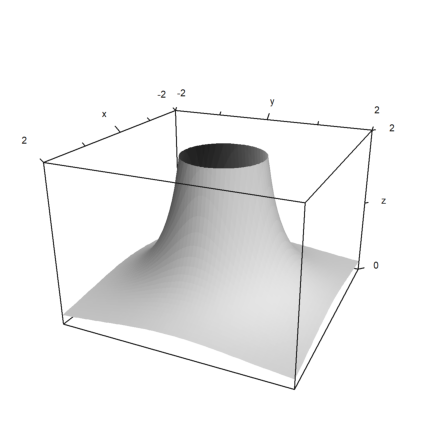
>plot3d("5*exp(-x^2-y^2)",r=2,<fscale,<scale,distance=13,height=50°, ...
   center=[0,0,-2],frame=3):
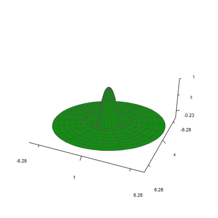
The parameter polar=true draws a polar plot. The function must still be a function of x and y.
>function f(r) := exp(-r/2)*cos(r); ...
 plot3d("f(x^2+y^2)",>polar,scale=[1,1,0.4],r=2pi,frame=3):
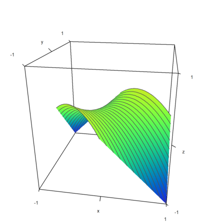
The parameter rotate rotates a function in x around the x-axis.
>plot3d("x^2+1",a=-1,b=1,rotate=true,grid=5):
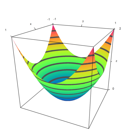
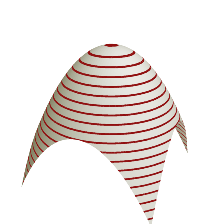
Euler can draw the heights of functions on a plot with shading.
The default is level="auto", which computes some level lines automatically. As you see in the plot, the levels are in fact ranges of levels.
>plot3d("exp(x*y)",angle=100°,>contour,color=green):
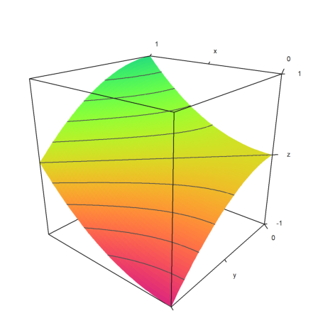
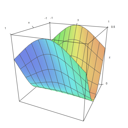
The default shading uses a gray color. But a spectral range of colors is also available.
For the following plot, we use the default spectral scheme and increase the number of points to get a very smooth look.
>plot3d("x^2+y^2",>spectral,>contour,n=100):
Instead of automatic level lines, we can also set values of the level lines. This will produce thin level lines instead of ranges of levels.
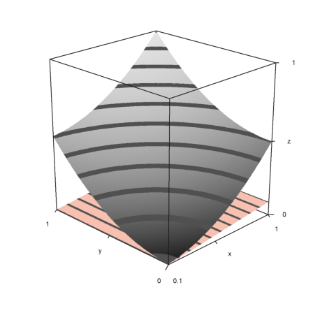
>plot3d("x^2-y^2",0,1,0,1,angle=220°,level=-1:0.2:1,color=redgreen):
In the following plot, we use two very broad level bands from -0.1 to 1, and from 0.9 to 1. This is entered as a matrix with level bounds as columns.
Moreover, we overlay a grid with 10 intervals in each direction.
>plot3d("x^2+y^3",level=[-0.1,0.9;0,1], ...
   >spectral,angle=30°,grid=10,contourcolor=gray):
In the following example, we plot the set, where
![]()
We use a single thin line for the level line.
>plot3d("x^y-y^x",level=0,a=0,b=6,c=0,d=6,contourcolor=red,n=100):
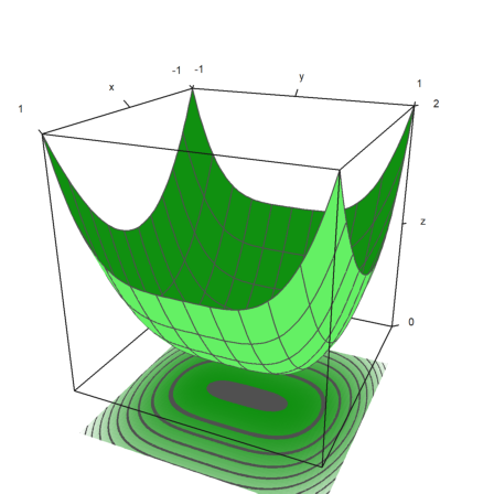
It is possible to show a contour plane below the plot. A color and distance to the plot can be specified.
>plot3d("x^2+y^4",>cp,cpcolor=green,cpdelta=0.2):
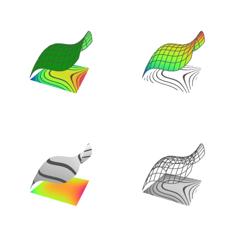
Here are a few more styles. We always turn off the frame, and use various color schemes for the plot and the grid.
>figure(2,2); ...
 expr="y^3-x^2"; ...
 figure(1);  ...
   plot3d(expr,<frame,>cp,cpcolor=spectral); ...
 figure(2);  ...
   plot3d(expr,<frame,>spectral,grid=10,cp=2); ...
 figure(3);  ...
   plot3d(expr,<frame,>contour,color=gray,nc=5,cp=3,cpcolor=greenred); ...
 figure(4);  ...
   plot3d(expr,<frame,>hue,grid=10,>transparent,>cp,cpcolor=gray); ...
 figure(0):
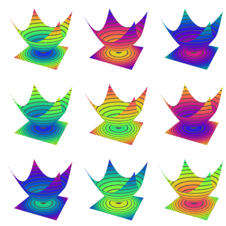
There are some other spectral schemes, numbered from 1 to 9. But you can also use the color=value, where value
>figure(3,3); ...
 for i=1:9;  ...
   figure(i); plot3d("x^2+y^2",spectral=i,>contour,>cp,<frame,zoom=4);  ...
 end; ...
 figure(0):
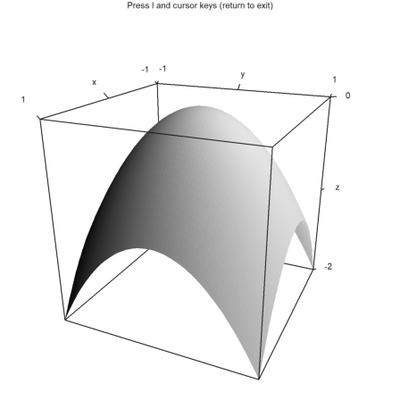
The light source can be changed with l and the cursor keys during the user interaction. It can also be set with parameters.
Note that the program does not make a difference between the sides of the plot. There are no shadows. For this you would need Povray.
>plot3d("-x^2-y^2", ...
   hue=true,light=[0,1,1],amb=0,user=true, ...
   title="Press l and cursor keys (return to exit)"):
The color parameter changes the color of the surface. The color of the level lines can also be changed.
>plot3d("-x^2-y^2",color=rgb(0.2,0.2,0),hue=true,frame=false, ...
   zoom=3,contourcolor=red,level=-2:0.1:1,dl=0.01):
The color 0 gives a special rainbow effect.
>plot3d("x^2/(x^2+y^2+1)",color=0,>hue,grid=10):
The surface can also be transparent.
>plot3d("x^2+y^2",>transparent,grid=10,wirecolor=red):
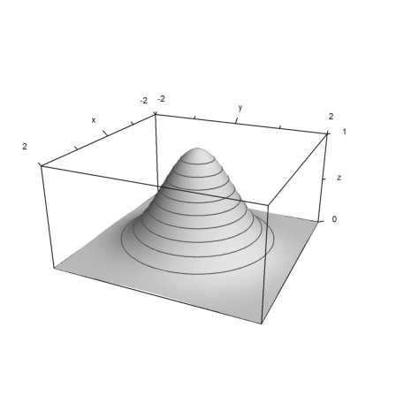
Function plots can be clipped. This is done with the "limits" vector and applies to the z-values. It looks better than a simple plateau which can be generated by "min(f(x,y),zmax)". The frame will be according to the plot data still, unless "zlim" is provided.
>plot3d("min(1/(x^2+y^2),3)",r=2,limits=[0,2],>hue,zlim=[0,2]):
The limits work for given values. The values are also used to compute the levels.
>x=linspace(-1,1,100); y=x'; z=x*y; ...
 plot3d(x,y,z,values=x+y,levels=-1:0.1:1,>spectral, ...
   limits=[-1,1],angle=10°):
Plots with x-y-z-values are scaled uniformly in each direction. If you want a non-uniform scaling, you can set the scaling for each dimension.
>x=linspace(-2,2,100); y=x'; z=exp(-x^2-y^2); ...
 plot3d(x,y,z,>hue,scale=[1,1,2],levels=0:0.1:1):
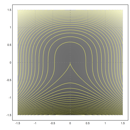
Contour plots are also possible in the plane using plot2d. Such plots plot the solutions of functions of two variables.
Let us plot the set
![]()
We can add a shading to the plot, which indicated large and small values, and we can change the color and the width of the contour.
>plot2d("x^2+y^3",level=-10:0.2:10,r=1.5,>hue, ...
   contourcolor=yellow,n=100):
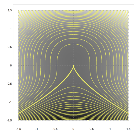
We can emphasize contour lines using >add.
>plot2d("x^2+y^3",level=0,>add, ...
   contourcolor=yellow,color=yellow,contourwidth=3,n=100):
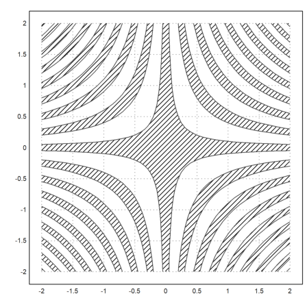
It is possible to draw level sets of the form
![]()
The bounds of the level sets are in two rows of the levels matrix. We can build such a matrix by adding a row vector to a 2x1 column vector.
>plot2d("x*y",r=2,levels=(-4:0.5:4)+[-0.1;0.1],style="/"):
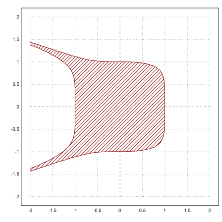
For an easier example, we plot the set
![]()
We use a data matrix for this.
>x=-2:0.1:2; y=x'; ...
   plot2d(x^3+y^6,a=-2,b=2,c=-2,d=2, ...
     levels=[-1;1],color=red,contourcolor=red,style="/"):
There are also implicit plots in three dimensions. The solutions of
![]()
can be visualized in cuts parallel to the x-y-, the x-z- and the y-z-plane.
Add these values, if you like. In the example we plot
![]()
>plot3d("x^2+y^3+z*y-1",r=5,implicit=3):
Just as plot2d, plot3d accepts data. You need to specify matrices x,y,z with the coordinates of the plane.
![]()
Since x,y,z are matrices, we assume that (t,s) run through a square grid. As a result, you can plot images of rectangles in space.
You can use the Euler matrix language to produce the coordinates effectively.
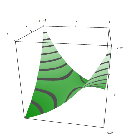
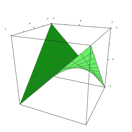
Here is an example, which is the graph of a function.
>t=-1:0.1:1; s=(-1:0.1:1)'; plot3d(t,s,t*s,grid=10):
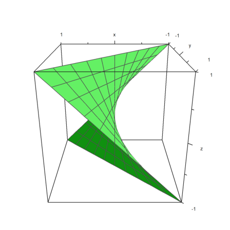
However, we can make all sorts of surfaces. Here is the same surface as a function
![]()
>plot3d(t*s,t,s,angle=180°,grid=10):
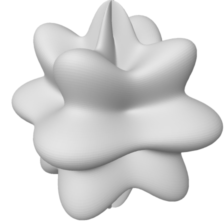
With more effort, we can produce many surfaces.
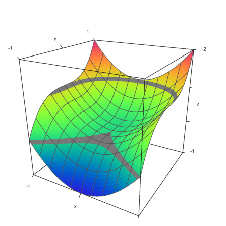
In the following example we make a shaded view of a distorted ball. The usual coordinates for the ball are
![]()
with
![]()
We distort this with a factor
![]()
>t=linspace(0,2pi,320); s=linspace(-pi/2,pi/2,160)'; ...
 d=1+0.2*(cos(4*t)+cos(8*s)); ...
 plot3d(cos(t)*cos(s)*d,sin(t)*cos(s)*d,sin(s)*d,hue=1, ...
   light=[1,0,1],frame=0,zoom=5):
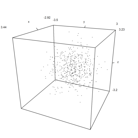
To plot point data in the space, we need three vectors for the coordinates of the points.
The styles are just as in plot2d with points=true;
>n=500;  ...
   plot3d(normal(1,n),normal(1,n),normal(1,n),points=true,style="."):
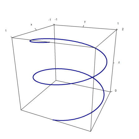
For curves in the plane we use a sequence of coordinates and the parameter wire=true.
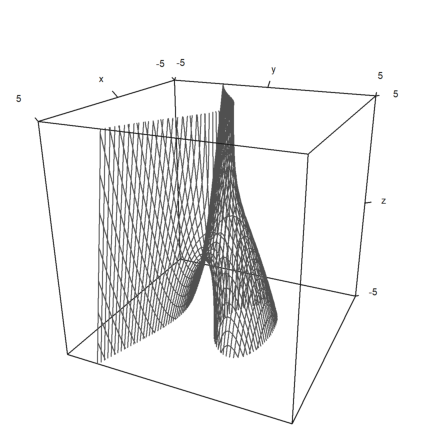
>t=linspace(0,4pi,1000); plot3d(cos(t),sin(t),t/2pi,>wire, ...
   linewidth=3,wirecolor=blue):
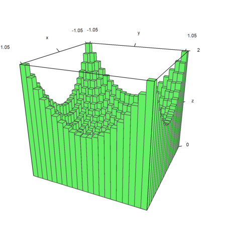
Bar plots are possible too. For this, we have to provide
z can be larger, but only nxn values will be used.
In the example, we first compute the values. Then we adjust x and y, so that the vectors center at the values used.
>x=-1:0.1:1; y=x'; z=x^2+y^2; ...
 xa=(x|1.1)-0.05; ya=(y_1.1)-0.05; ...
 plot3d(xa,ya,z,bar=true):
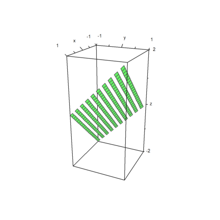
It is possible to split the plot of a surface in two or more parts.
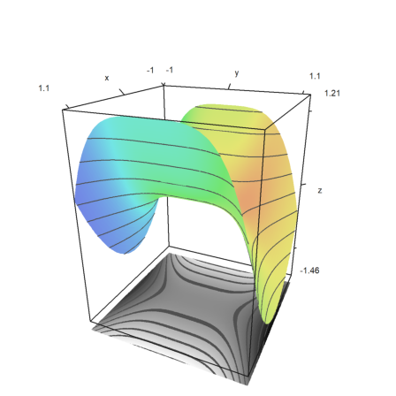
>x=-1:0.1:1; y=x'; z=x+y; d=zeros(size(x)); ...
 plot3d(x,y,z,disconnect=2:2:20):
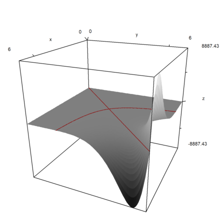
If load or generate a data matrix M from a file and need to plot it in 3D you can either scale the matrix to [-1,1] with scale(M), or scale the matrix with >zscale. This can be combined with individual scaling factors which are applied additionally.
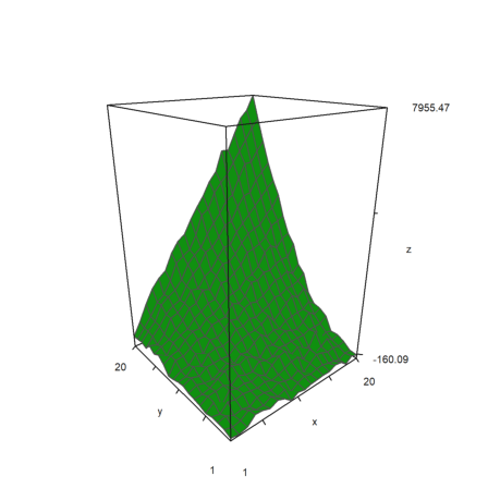
>i=1:20; j=i';  ...
 plot3d(i*j^2+100*normal(20,20),>zscale,scale=[1,1,1.5],angle=-40°,zoom=1.8):
The plot3d function is nice to have, but it does not satisfy all needs. Besides more basic routines, it is possible to get a framed plot of any object you like.
Though Euler is not a 3D program, it can combine some basic objects. We try to visualize a paraboloid and its tangent.
>function myplot ...
   y=0:0.01:1; x=(0.1:0.01:1)';
   plot3d(x,y,0.2*(x-0.1)/2,<scale,<frame,>hue, ..
     hues=0.5,>contour,color=orange);
   h=holding(1);
   plot3d(x,y,(x^2+y^2)/2,<scale,<frame,>contour,>hue);
   holding(h);
 endfunction
Now framedplot() provides the frames, and sets the views.
>framedplot("myplot",[0.1,1,0,1,0,1],angle=-45°, ...
   center=[0,0,-0.7],zoom=6):
In the same way, you can plot the contour plane manually. Note that plot3d() sets the window to fullwindow() by default, but plotcontourplane() assumes that.
>x=-1:0.02:1.1; y=x'; z=x^2-y^4;
>function myplot (x,y,z) ...
   zoom(2);
   wi=fullwindow();
   plotcontourplane(x,y,z,level="auto",<scale);
   plot3d(x,y,z,>hue,<scale,>add,color=white,level="thin");
   window(wi);
   reset();
 endfunction
>myplot(x,y,z):
Euler can use frames to pre-compute the animation.
One function, which makes use of this technique is rotate. It can change the angle of view and redraw a 3D plot. The function calls addpage() for each new plot. Finally it animates the plots.
Please study the source of rotate to see more details.
>function testplot () := plot3d("x^2+y^3"); ...
 rotate("testplot"); testplot():