In this tutorial, we demonstrate how to solve Analysis problems in Euler numerically. Many problems do not have a symbolic solutions, or are too large. Then we need numerical methods.
Let us start with numerical integrals. To see the accuracy, we switch to the longest possible format.
>longestformat;
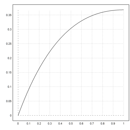
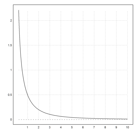
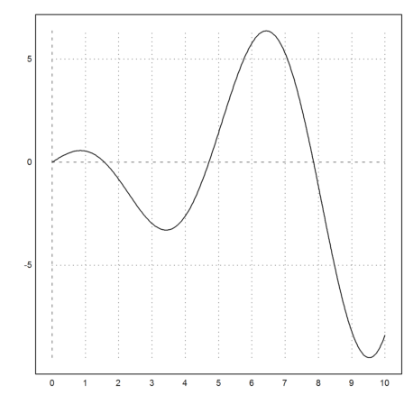
Let us try the following integral.
![]()
First we plot the function.
>plot2d("exp(-x)*x",0,1):
In this simple case, Maxima can compute the exact integral symbolically. We evaluate the result numerically.
>&integrate(exp(-x)*x,x,0,1), %()
                                     - 1
                              1 - 2 E

0.2642411176571153
The default integration is an adaptive Gauss quadrature.
>integrate("exp(-x)*x",0,1)
0.2642411176571153
It works very well, even for singular functions. The non-adaptive Gauss method is much faster and takes only 10 function evaluations.
>integrate("sqrt(x)",0,1), gauss("sqrt(x)",0,1)
0.6666666666666667
0.6667560429365088
For smooth functions, both deliver the same accuracy.
>integrate("x*exp(-x)",0,1), gauss("x*exp(-x)",0,1), 1-2/E
0.2642411176571153
0.2642411176571154
0.2642411176571153
The function Romberg is very accurate for smooth functions. But it is slower.
>romberg("exp(-x)*x",0,1)
0.2642411176571154
The Simpson rule is good for functions, which are not so smooth. In general, the results are inferior, and the algorithm uses much more evaluations of the function. To get the same accuracy, we need 2000 evaluations.
>simpson("exp(-x)*x",0,1,n=1000)
0.2642411176571147
The Simpson method is useful, if a vector of data is given, not a function. We can sum the Simpson integral directly using the Simpson factors 1,4,2,...,2,4,1.
>n=2000; x=linspace(0,1,n); y=exp(-x)*x; sum(y*simpsonfactors(n/2))/n/3
0.2642411176571147
The Simpson method has a variant, which returns the values of the integral at all points.
>{x,y}=simpson("sin(x)",0,2pi,200,>allvalues); plot2d(x,y):
We can also use Maxima via mxmintegrate() to find this integral exactly. For more information, see the introduction to Maxima.
>mxmintegrate("exp(-x)*x",0,1)
0.2642411176571153
Critical functions, like exp(-x^2), need more intervals for the Gauss integration. This function tends to 0 very quickly for large |x|. We use 10 sub-intervals, with a total of 100 evaluations of the function. This is the default for the integrate function.
>gauss("exp(-x^2)",-10,10,10)
1.772453850904878
The result is not bad.
>sqrt(pi)
1.772453850905516
However, the solid Romberg method works too.
>romberg("exp(-x^2)",-10,10)
1.772453850905285
The adaptive Gauss routine works even better.
>integrate("exp(-x^2)",-10,10)
1.772453850905516
Maxima knows this infinite integral, of course.
>&integrate(exp(-x^2),x,-inf,inf)
sqrt(pi)
If we integrate to other values, Maxima expresses the result in terms of the Gauß distribution.
>&integrate(exp(-x^2),x,0,1), &float(%)
                           sqrt(pi) erf(1)
                           ---------------
                                  2


                          0.7468241328124269
This is the numerical result of Euler.
>integrate("exp(-x^2)",0,1)
0.746824132812427
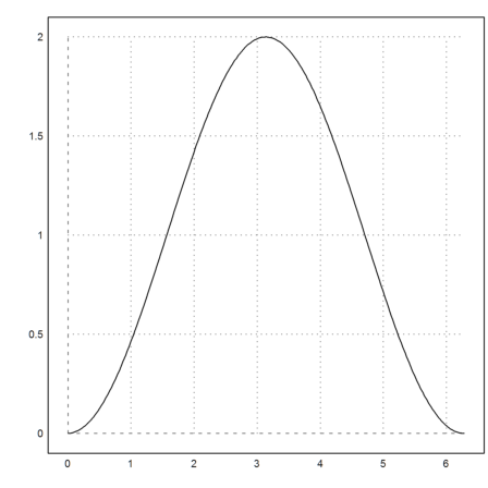
We try another example.
![]()
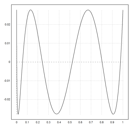
Let us plot the sinc function from -pi to 2pi.
>plot2d("sinc(x)",a=-pi,b=2pi):
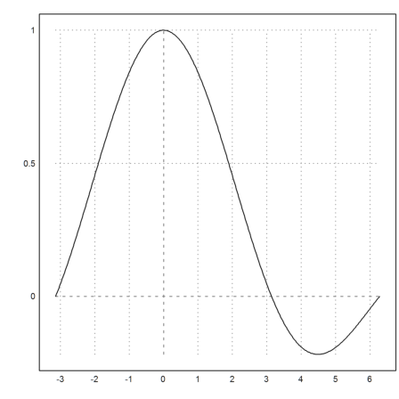
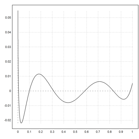
We are going to draw the integral of this function from 0 to x. So we define a function doing an integration for each x.
It is essential to use map here, since f does not work for vectors x automatically.
>function map f(x) := gauss("sinc(x)",0,x)
The plot of the integral does a lot of work. But it is still surprisingly fast.
>plot2d("f",a=0.01,b=2*pi):

Using a cumulative Simpson sum is much faster, of course.
>x=linspace(0,2*pi,500); y=sinc(x); ...
   plot2d(x,cumsum(y*simpsonfactors(250))*(2pi/500)/3):
Of course, the derivative of f() is sinc(). We test that with the numerical differentiation of Euler.
>diff("f",2), sinc(2)
0.4546487134117229
0.4546487134128409
The first zero of sinc() is pi.
>diff("f",pi)
1.914752621372156e-012
Sometimes, we have a function depending on a parameter like
![]()
>function g(x,a) := x^a/a^x
We can now use an expression for the gauss function and a global value a.
>a=0.5; gauss("g(x,a)",0,1)
1.026961217763892
But in functions, we do not want to use global variables.
How do we set this parameter for the gauss function in this case? The solution is to use a semicolon parameter. All parameters after the semicolon are passed to the function "f".
>gauss("g",0,1;0.5), gauss("g",0,1;0.6),
1.026961217763892
0.8631460080035323
To plot such a function depending on the value a, we should define a function first.
>function ga (a) := gauss("g",0,1;a);
Now we plot
![]()
>plot2d("ga",0.2,10):
It might be easier to use call collections. A call collection contains a function and its parameters in a list.
>gauss({{"g",0.5}},0,1)
1.026961217763892
The same trick works for expressions. Expressions can see global variables, or variables passed to the evaluation. For functions like integrate(expr,...) we can pass a local variable by reference as a semicolon parameter. Note, that values can not be used, since they have no name.
This allows to define local functions for integration as in the next example where we define the function
![]()
We need to vectorize the function with "map", since it would not work for vector input.
>function map F(x;a) ...
 expr="1/(1+x^a)";
 return integrate({{expr,a}},0,x)
 endfunction
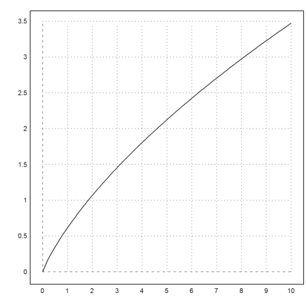
Let us evaluate the function in the interval [0,10] for a=3.
>t=0:0.1:10; s=F(t,3); plot2d(t,s):
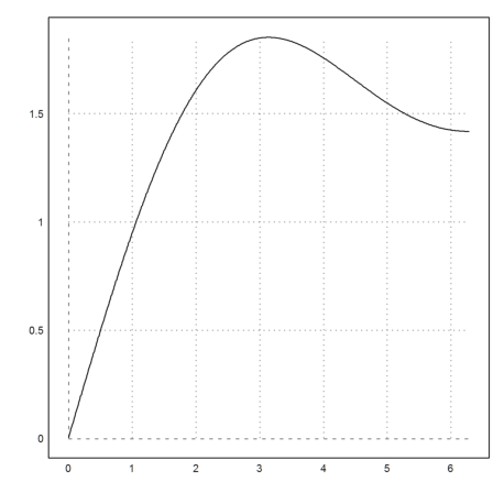
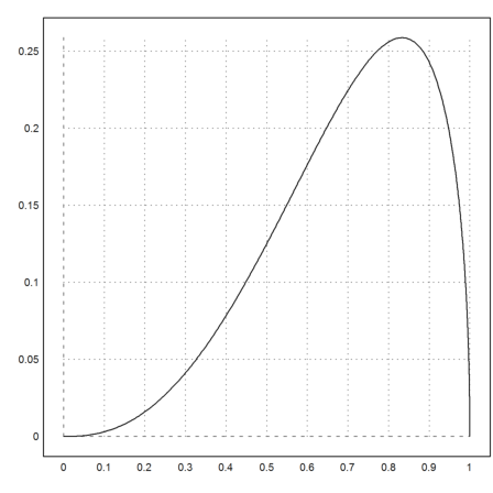
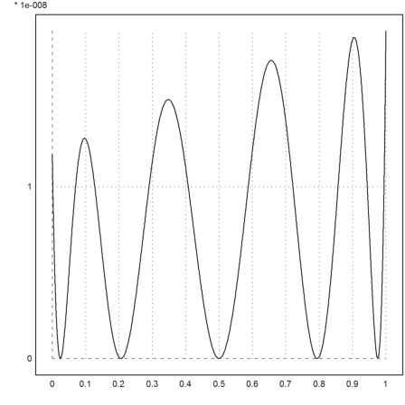
As an example, we want to integrate the following function, which appears as a weight function in orthogonal polynomials.
>function fbeta(x,a,b) := x^(a-1)*(1-x)^(b-1)
A specific example looks like this.
>plot2d("fbeta(x,3.5,1.5)",0,1):
The adaptive Runge method can be used to compute integrals. It is the method of choice for adaptive integration in Euler.
>adaptiveint("fbeta(x,3.5,1.5)",0,1)
0.1227184630325045
It has the alias "integrate" with method=1.
>integrate("fbeta(x,3.5,1.5)",0,1,method=1)
0.1227184630325045
To count the number of function evaluations, we define a help function.
>function fbetacount(x,a,b) ...
 global fcount;
 fcount=fcount+1;
 return fbeta(x,a,b)
 endfunction
The result is that the function is called over 5000 times, far more than the Gauß scheme.
>fcount=0; adaptiveint("fbetacount(x,3.5,1.5)",0,1), fcount,
0.1227184630325045
2650
The adaptive Gauss method does a very good job here.
>fcount=0; integrate("fbetacount(x,3.5,1.5)",0,1), fcount,
0.1227184630311863
1830
Euler can compute this value with the Beta function.
>beta(3.5,1.5)
0.1227184630308513
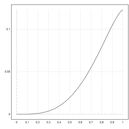
To get all intermediate points of the anti-derivative we must call adaptiverunge directly.
>t:=linspace(0,1,100); s:=adaptiverunge("fbeta(x,3.5,1.5)",t,0); ...
 plot2d(t,s):
The default function to solve an equation of one variable is solve. It needs an approximation of the zero to start the iteration. The method used is the secant method.
>solve("cos(x)-x",1)
0.7390851332151607
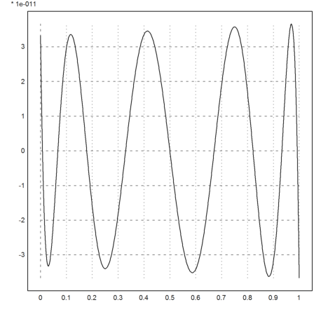
In the following plot, we see, that the function
![]()
has the value 1 close to x=5.
>plot2d("x*cos(x)",0,10):
So we solve for the target value y=1 with starting point 5.
>solve("x*cos(x)",5,y=1)
4.917185925287132
The bisection method is more stable than the secant method. It needs an interval such that the function has different signs at the ends of the interval.
>bisect("exp(-x)-x",0,2)
0.5671432904100584
For problematic cases there is the secantin() function, which does not leave the interval. The secant function would run into negative arguments here.
>secantin("x^x",0,0.2,y=0.9)
0.03006536848961514
The Newton method needs a derivative. We can use Maxima to provide a derivative. The function mxmnewton calls Maxima once for this.
>mxmnewton("exp(-x^2)-x",1)
0.6529186404192048
If we need the derivative more often, we should compute it as a symbolic expression.
>expr &= exp(x)+x; dexpr &= diff(expr,x);
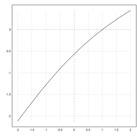
Then we can write a function to compute the inverse of
![]()
The Newton method solves f(x)=s very quickly.
>function map g(s) := newton(expr,dexpr,s,y=s); ...
 plot2d("g",-2,2,n=10):
For functions of several parameters, like the following, we can use solve() to solve for one of the variables with the following procedure.
>function h(a,b,c) := a*exp(b)-c*sin(b);
Now we solve for c=x. The variables a and b must be global, however.
>longformat; a=1; b=2; c=solve("h(a,b,x)",1)
8.12611570312
Let us check the result.
>h(a,b,c)
0
This does not work inside functions, since local variables to functions are not found by solve. So we use a function in x with additional parameters.
>function h2(x,a,c) := h(a,x,c)
We can use semicolon parameters to pass a and c for the function h2. For more information about semicolon parameters see the introduction about programming. As a starting value, we take a simply.
>function test(a,c) := solve("h2",a;a,c)
>b=test(1,2)
-326.725635973
Let us check this.
>h(1,b,2)
0
To compute maximal values, there is the function fmax(). As parameters, it needs the endpoints of an interval and a function or expression, using the Golden Ratio algorithm. This works for all concave functions.
Let us find the maximum of the integral of the sinc() function.
>fmax("f",1,2*pi)
3.14159262875
Of course, this is pi. The maximum is not completely accurate, since computing the maximum is an ill posed problem. I.e., for x-values close to pi the function will have almost the same values.
>pi
3.14159265359
We can also compute the minimum.
>fmin("sinc(x)",pi,2*pi)
4.49340944137
Maxima can compute the derivative for us, and we can solve it numerically. This is much more accurate.
>solve(&diff(sin(x)/x,x),4.5)
4.49340945791
The solution cannot be expressed exactly. So Maxima does not get an answer here.
>&solve(diff(sin(x)/x,x),x)
                                  sin(x)
                             [x = ------]
                                  cos(x)
Euler does also have advanced interval methods, which yield guaranteed inclusions for the solution.
One example is ibisect(). The guaranteed inclusion shows that our numerical solver is rather good.
>ibisect(&diff(sin(x)/x,x),4,5)
~4.493409457905,4.493409457913~
Assume, we want to solve
![]()
simultaneously. So we seek the zero of the following function.
>function f([x,y]) := [x^2+y^2-10,x*y-3]
We define the function with vector parameters. It can be used for two real arguments x,y or for vectors [x,y]
There are various method to solve f=0 in Euler. E.g., the Newton method uses the Jacobian of f. We do not discuss this here. Have a look at the following tutorial.
The Broyden method is a Quasi-Newton method, which works almost as good as the Newton method.
>broyden("f",[1,0])
[3, 1]
We find the solution x=3 and y=1.
If we start at a place with x=y, we get an error, since the Jacobian is non-singular. The Broyden method uses an approximation to the Jacobian.
The Nelder method uses a minimization routine with simplices. It works very stable and fast, if the number of variables is not too high.
We need a function norm(f(v)), since Nelder seeks minimal values.
>function fnorm(v) := norm(f(v))
>nelder("fnorm",[1,0])
[3, 1]
In this simple example, Maxima finds all solutions.
>&solve([x^2+y^2=10,x*y=3])
       [[y = - 3, x = - 1], [y = 1, x = 3], [y = - 1, x = - 3],
                                                       [y = 3, x = 1]]
The Powell minimization routine finds the same minimum.
>powellmin("fnorm",[1,0])
[3, 1]
Interpolation is a tool to determine a function, which has given values at given points. Approximation is for fitting a curve to a function. We demonstrate both.
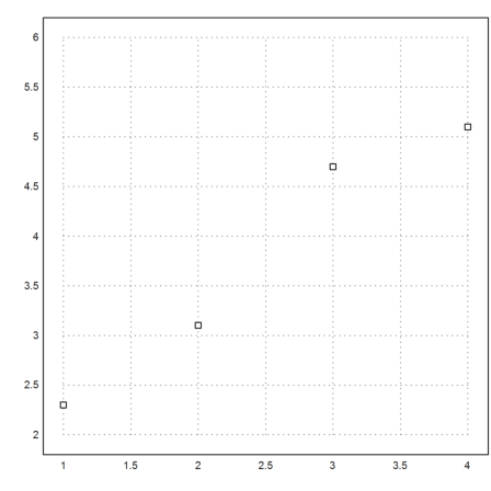
Assume, we have four data points.
>xp=[1,2,3,4]; yp=[2.3,3.1,4.7,5.1];  ...
   plot2d(xp,yp,points=true,a=1,b=4,c=2,d=6):
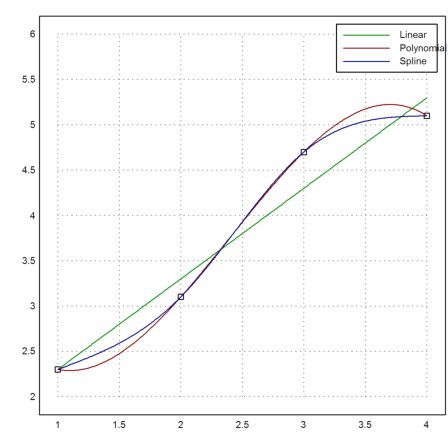
We can fit a linear function to these data. The function is chosen such that the sum of all squared errors is minimal (least squares fit).
>p=polyfit(xp,yp,1); plot2d("evalpoly(x,p)",color=green,add=true);
We can also try to run a polynomial of degree 3 through these points.
>d=divdif(xp,yp); plot2d("evaldivdif(x,d,xp)",add=true,color=red);
Another choice would be natural spline.
>s=spline(xp,yp); plot2d("evalspline(x,xp,yp,s)",add=true,color=blue); ...
   labelbox(["Linear","Polynomial","Spline"],colors=[green,red,blue]):
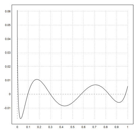
For another example, we interpolate the exponential function in [0,1] using a polynomial of degree 8 in the zeros of the Chebyshev polynomial.
The error is about 3*10^-11. This is very close to the optimal error we can achieve.
>xp=chebzeros(0,1,9); yp=exp(xp); d=divdif(xp,yp); ...
 plot2d("evaldivdif(x,d,xp)-exp(x)",0,1):
We can also use Hermite-Interpolation, either with data or with a function. In the following example, we use a function. The function must be able to return the values, and all needed derivatives.
First we need a vector of Chebyshev zeros, with each one duplicated twice.
>xp2=multdup(chebzeros(0,1,5),2)
[0.0244717418524,  0.0244717418524,  0.206107373854,  0.206107373854,
0.5,  0.5,  0.793892626146,  0.793892626146,  0.975528258148,
0.975528258148]
Now the function f, and the derivative function df.
>function f(x) &= exp(-x^2);
We use Maxima at compile time with &:...
>function df(x,n) ...
 if n==0 then return f(x);
 else return &:diff(f(x),x);
 endif;
 endfunction
The function hermite() returns the divided differences as usual.
>d=hermiteinterp(xp2,"df");
Now the error is always positive. The approximation is one-sided, i.e., the error is non-negative everywhere.
>plot2d("f(x)-interpval(xp2,d,x)",0,1):
Euler can also compute the best approximation in the sup-norm using the Remez algorithm.
>xp=equispace(0,1,100); yp=sqrt(xp); ...
 {t,d}=remez(xp,yp,5); ...
 plot2d("interpval(t,d,x)-sqrt(x)",0,1):
Compare this to the least square fit.
>p=polyfit(xp,yp,5); ...
 plot2d("evalpoly(x,p)-sqrt(x)",0,1):
Using a non-linear fit, we can find the polynomial approximation in any functional norm. Starting from p, we can improve the L1-norm.
>function model(x,p) := polyval(p,x); ...
 p1=modelfit("model",p,xp,yp,p=1); ...
 plot2d("evalpoly(x,p1)-sqrt(x)",0,1):
For more than a few dimension, multi-dimension is a tough subject and hard to compute. We demonstrate here, how Euler can integrate functions of two variables using the theorem of Fubini.
If we want to integrate in two variables numerically, we need to define two functions. First, let us use Maxima to compute the integral of a specific function over a unit square.
>function fxy (x,y) &= y^2*exp(y*x)
                                2  x y
                               y  E
Then we can integrate
![]()
symbolically.
>&integrate(integrate(fxy(x,y),x,0,1),y,0,1)
                                  1
                                  -
                                  2
To do that numerically in Euler, we define a function for the inner integral. Note that we pass y as additional parameter to fxy.
>function map f1(y) := integrate("fxy",0,1;y)
It is essential to let this function map, since it will not work for vectors y.
Then we integrate this. Note that the result is very accurate.
>integrate("f1",0,1)
0.5
For a general solution, we pass the function as an argument to the inner integral.
>function map gaussinner(y;f$,a,b,n=1) := gauss(f$,a,b,n;y)
Then we use this to compute the outer integral. The parameters after the semicolon ; for gauss are passed to gaussinner().
>function gausstwo (f$,a,b,c,d,n=1) := gauss("gaussinner",c,d,n;f$,a,b,n)
Check it with the known value
>gausstwo("fxy",0,1,0,1,n=20)
0.5
This function is already predefined in Euler using the simple Gauss integration, and it works for expressions too.
>gaussfxy("y^2*exp(y*x)",0,1,0,1,n=100)
0.5
Check with a more unstable function.
>function g(x,y) := x^y
>longest gaussfxy("g",0,1,0,1)
0.6932668572191346
The accuracy is not as good as we like. This is due to the singularity in x=y=0.
>longest log(2)
0.6931471805599453