We want to look at some differential equations and the numerical methods of Euler to solve these equations.
Reference for Differential Equations
To understand this tutorial, you should have an elementary knowledge about the programming language of Euler.
First, there is the Runge-Kutta method.
For an example, we take the initial value problem
![]()
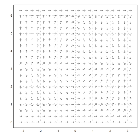
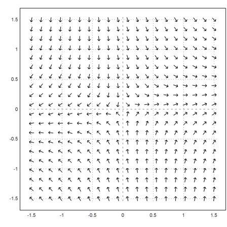
We want to compute and plot all values of the solution between -3 and 3. So we have to split the region in two, going back and forth from 0.
We first plot the vector field using the function "vectorfield". The functions needs an expression in x and y.
>vectorfield("x*y*sin(y)",-pi,pi,0,2pi,nx=20,ny=20,color=gray):
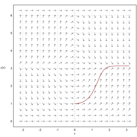
Then we compute and plot the right side of the solution. The Runge method computes values of the solution at given points. We need to supply a function or an expression, and an initial value.
The Runge method takes a vector of x-values and an initial value at x[1]. It returns the values at all points x[i] in a vector. We can plot the solution easily with these two vectors.
>t=0:0.01:pi; s=runge("x*y*sin(y)",t,1);  ...
   plot2d(t,s,color=red,>add,xl="x",yl="y(x)",<vertical):
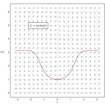
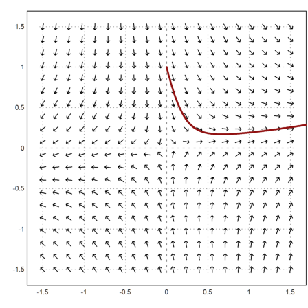
Add the solution from 0 to -3 to the plot, and the initial value.
>t=0:-0.01:-pi; s=runge("x*y*sin(y)",t,1);  ...
   plot2d(t,s,color=red,>add);  ...
   plot2d(0,1,color=red,>points,>add); ...
   textbox(latex("y'=x y \sin(y)",factor=1.5),0.4,0.2):
It is not necessary to return all the values in the function "runge". But then we have to tell the routine to use lots of intermediate points. In the following example, we get only two values with 500 lost intermediate values.
>runge("x*y*sin(y)",[0,10],1,500)
[1, 3.141592653589793]
To demonstrate other solvers we solve
![]()
with the solution
![]()
For critical problems, there is an adaptive version of the Runge method. It does not need intermediate steps.
We test the method by counting the evaluations of f(x,y). To do this, we use a function instead of an expression. Inside the function we increase a global count.
>function f(x,y) ...
 global count;
 count=count+1;
 return -x/(1+y);
 endfunction
Now, let us test the adaptive Runge method.
>longestformat;  ...
   count=0; adaptiverunge("f",[0,1.99],1)[-1], count,
-0.8002501564119474
993
This is very good for 1000 evaluations of f. The correct value is the following.
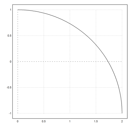
>function ysol(x) := sqrt(4-x^2)-1; ...
 ysol(1.99)
-0.8002501564456186
The function has a singularity at x=2.
>plot2d("ysol",0,2):
For comparison, we need 20000 function evaluations, and don't get the same accuracy with the Runge method.
>count=0; runge("f",[0,1.99],1,5000)[-1], count,
-0.8002501565525217
20000
Euler has also the LSODA method, which is the default for the ode function. This is an adaptive method, and it gets very good results with very few evaluations.
>count=0; ode("f",[0,1.99],1)[-1], count,
-0.8002501588030427
573
To increase the accuracy, we can add an epsilon and intermediate points. The LSODA algorithm interpolates the intermediate points with no evaluations of f. If epsilon is too small, it will fail. But 10^-13 seems to be okay for this problem.
>count=0; ode("f",linspace(0,1.99,10000),1,eps=1e-13)[-1], count,
-0.8002501565191461
534
Euler can also get a guaranteed inclusion for the solution of this differential equations.
The function mxmidgl calls Maxima to get a Taylor expansion of the equation of very high degree. It then uses the remainder formula to get an inclusion of the solution.
>mxmidgl("-x/(1+y)",linspace(0,1.99,1000),1)[-1]
~-0.800250156479,-0.800250156435~
The correct solution is indeed in this interval.
>ysol(1.99)
-0.8002501564456186
The function can also be used for integration by solving the differential equation
![]()
The function mxmiint uses this method.
>mxmiint("sin(x)/x",pi,2pi)
~-0.433785475849854,-0.433785475849821~
In many cases, Maxima delivers exact solutions. Let us try the initial value problem
![]()
The standard function of Maxima is ode2. To get the solution for an initial value, we use ic1.
>&ode2(y+x*'diff(y,x)=log(x)+1,y,x), sol &= ic1(%,x=1,y=1)
                              x log(x) + %c
                          y = -------------
                                    x


                               x log(x) + 1
                           y = ------------
                                    x
If you want to make a function of this solution, use the following trick.
>function ysol(x) &= y with sol
                             x log(x) + 1
                             ------------
                                  x
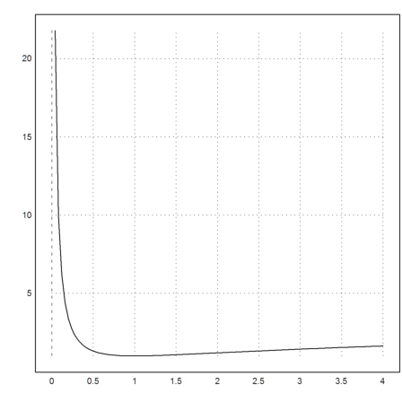
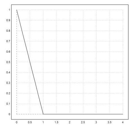
We can now plot this function.
>plot2d("ysol",0,4):
The numerical solution is the same.
>res := ode("(log(x)+1-y)/x",[1,2],1); ...
 longestformat; res[2], ysol(2)
1.193147180564709
1.193147180559945
We can try to solve the equation
![]()
in Maxima, but it does not really work.
>&x*y*sin(y)='diff(y,x); &ode2(%,y,x)
                       /                2
                       [    1          x
                       I -------- dy = -- + %c
                       ] y sin(y)      2
                       /
Looking at the integral, we see that we need to use a numerical approximation for the integral on the left side, and a further numerical approximation to solve I(y)=x^2/2 for y. We use the fast and stable Gauss method for the integral.
>function fi (y,x) := gauss("1/(x*sin(x))",1,y,20)-x
And the super-stable bisection method for the solution.
>function fy (x) := bisect("fi",1,pi;x^2/2)
Yet we can find the solution only in [-2,2]. The result is the same as with the Runge method in this range. The Runge-Kutta method seems to work better, and the Gauss integral becomes unstable.
>longestformat; fy(2), res=runge("x*y*sin(y)",[0,2],1,500); res[2]
3.103165883965475
3.103165883778106
For a second example, we solve the problem
![]()
Again the solution is implicit, and we need to solve it for y.
>&ode2('diff(y,x)=-x/(1+y),y,x), sol &= rhs(solve(%,y)[2])
                            2          2
                         - y  - 2 y   x
                         ---------- = -- + %c
                             2        2


                              2
                      sqrt(- x  - 2 %c + 1) - 1
To find the constant, we can use the standard solver of Maxima instead of ic1.
>&solve((sol with x=0)=1), function ysol(x) &= sol with %
                                      3
                              [%c = - -]
                                      2


                                     2
                           sqrt(4 - x ) - 1
Solving
![]()
numerically requires a rewrite into a system of equations.
![]()
We write a function f(x,u).
>function f(t,u) := [u[2],-u[1]^2]
The time variable t is not used in this function in this case.
Now we solve
![]()
with the Runge method.
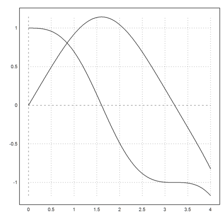
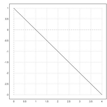
>t=linspace(0,4,500); s=runge("f",t,[0,1]);
The result is a matrix with two rows y and y'. We plot both into one plot.
>plot2d(t,s):
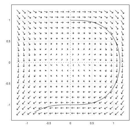
We can plot the vector field for this, since the time does not matter. Note that vector fields in the plane need two expressions in x and y, one for each component of the vector at (x,y).
>vectorfield2("y","-x^2",r=1.2); plot2d(s[1],s[2],>add):
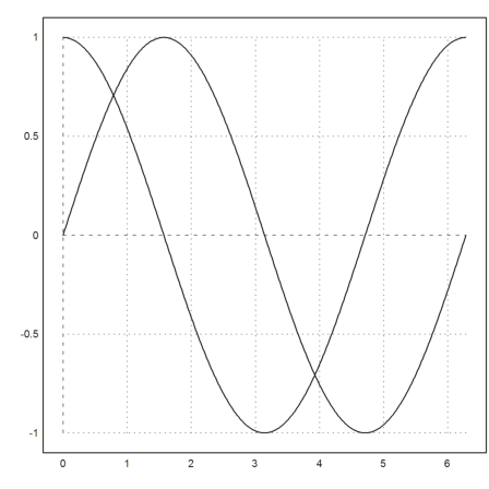
We can also use a vector parameter. We solve
![]()
>function f(x,[y1,y2]) := [y2,-y1]; ...
 x=linspace(0,2pi,500); plot2d(x,ode("f",x,[0,1])):
A linear system is of the form
![]()
>A = [1,0.5;0.5,-2]; function f(x,u) := A.u;
We can use Maxima to derive a formula for the vector field with
![]()
>Axy &= @A.[x,y]
                           [  0.5 y + x  ]
                           [             ]
                           [ 0.5 x - 2 y ]
Then draw the hyperbolic vector field.
>vectorfield2(&Axy[1],&Axy[2],r=1.5,>normalize):
We now compute the track of a solution for t=0 to t=10.
>t=linspace(0,10,1000); s=runge("f",t,[0;1]); ...
 plot2d(s[1],s[2],color=red,thickness=3,>add):
The exact solution of such a differential equation is
![]()
Euler has a function to apply an analytic function to a matrix, which decomposes the matrix and applies the function to the eigenvalues.
>matrixfunction("exp",10*A).[0;1]
      7839.642977982564
      1272.198919023391
Compare to the numerical result.
>s[,-1]
      7839.642968419197
      1272.198917471471
Maxima can derive a formula for this solution.
>function u(t) &= matrixexp(t*@A).[0;1];
The formula is
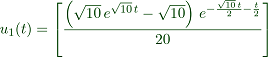
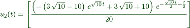
To print this in the comment, use
 maxima: u[1](t) = u(t)[1]
 maxima: u[2](t) = u(t)[2]
>u(10)
       7839.64297798256
      1272.198919023391
The following example
![]()
is very difficult to solve with the Runge method.
>c=1e-5; x=0:0.1:4; plot2d(x,ode("-y/(c+y)",x,1)):
But the LSODA algorithm, which is used in ode() by default, switches to a different formula if the equations becomes "stiff".
If we solve this with the ordinary Runge method for small c, we get essentially the solution of
![]()
>c=1e-5; x=0:0.1:4; plot2d(x,runge("-y/(c+y)",x,1)):
In many cases, this kind of equation simply wants to simulate a change of the behavior of f(x,y). It might be far better to use cases.
>function f(x,y) ...
   global c;
   if y>0 then return -y/(c+y);
   else return 0
 endfunction
The solution is not perfect, since it equals a small negative constant c>1. But it far easier to compute, and we can chop away the parts were y<0 in the plot.
>c=1e-5; x=0:0.01:4; plot2d(x,max(runge("f",x,1),0)):

Here is another example. We solve
![]()
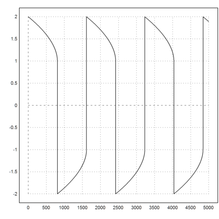
This is a stiff equation. The simple Runge algorithm does not work. But LSODA can handle this very well.
Note that we defined f() with a vector parameter.
>function f(x,[y1,y2]) := [y2,1000*(1-y1^2)*y2-y1]; ...
 x=0:0.01:5000; y=ode("f",x,[2,0]); plot2d(x,y[1]):
Let us solve a boundary value problem numerically. The differential equation is
![]()
We rewrite that in two dimensions and get
![]()
We want the boundary values
![]()
We have to rewrite the equation into a system of equations.
>function f(x,y) := [y[2],x*y[1]]
We can use the LSODA algorithm to solve this for
![]()
>y=ode("f",[0,1],[1,0]); y[1,2]
1.172299970082665
The next step is to solve for the boundary values. We set up a function, which has a zero in the solution by taking y'(0) as a parameter and y(1)-1 as the function value.
>function g(a) ...
 t=0:0.001:1;
 y=ode("f",[0,1],[1,a]);
 return y[1,2]-1;
 endfunction
We know already g(0)>0, and we see g(-2)<0.
>g(0), g(-2),
0.1722999700826648
-1.99837932614611
Thus the secant method yields the desired value for y'(0). This is called the "Shooting Method".
>a=secant("g",-2,2)
-0.1587521200144439
A final plot of the answer.
>t=0:0.05:1; y=ode("f",t,[1,a]); plot2d(t,y[1]):
Here is a more complex boundary value problem, which can be solved analytically in Maxima.
![]()
>&ode2('diff(y,x,2)+y=sin(x),y,x),  ...
 function f(x) &= y with bc2(%,x=0,y=0,x=%pi/2,y=-1)
                                 x cos(x)
                y = %k1 sin(x) - -------- + %k2 cos(x)
                                    2


                                    x cos(x)
                         - sin(x) - --------
                                       2
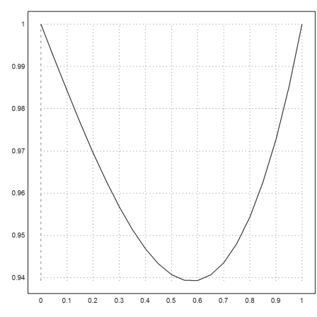
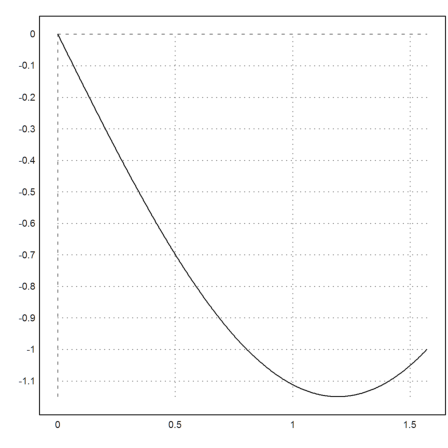
Let us plot the solution to this boundary value problem.
>plot2d(f,0,pi/2):
The correct derivative in 0 is -3/2.
>&diffat(f(x),x=0)
                                   3
                                 - -
                                   2
Let us try the shooting method.
>function f(x,y) := [y[2],sin(x)-y[1]]
The function g must be modified as follows.
>function g(a) ...
 y=ode("f",[0,pi/2],[0,a]);
 return y[1,2]+1;
 endfunction
Now
>g(0), g(-2),
1.500000000004345
-0.5000000000005538
And we do indeed find the correct derivative.
>a := bisect("g",-2,0)
-1.50000000000091