Euler Math Toolbox is very good for simulating random events. In this demo, I want to try a few examples.
Let us start with the simple normal distribution. We simulate a 1000-5-normal distributed random variable a million times. For this, we use the function normal(m,n), which generates a matrix of 0-1-distributed values, or normal(n) which defaults to m=1. To get a 5000-5-distribution, we use simple arithmetic with the matrix language of Euler.
>n=1000000; x=normal(n)*5+1000;
There is also the function randnormal(n,m,mean,dev), which we might use. This function obeys to the naming scheme "rand..." for random generators.
>n=1000000; x=randnormal(1,n,1000,5);
The first 10 values of x are the following.
>x[1:10]
[998.573,  1004.16,  1003.21,  1000.91,  1003.04,  987.759,  1002.54,
1007,  1002.05,  1001.67]
The distribution can easily be plotted with the >distribution flag of plot2d. I will show you in a minute how this can be done manually.
Let us add the expected density of the normal distribution.
>plot2d(x,>distribution);  ...
   plot2d("qnormal(x,1000,5)",color=red,thickness=2,>add):
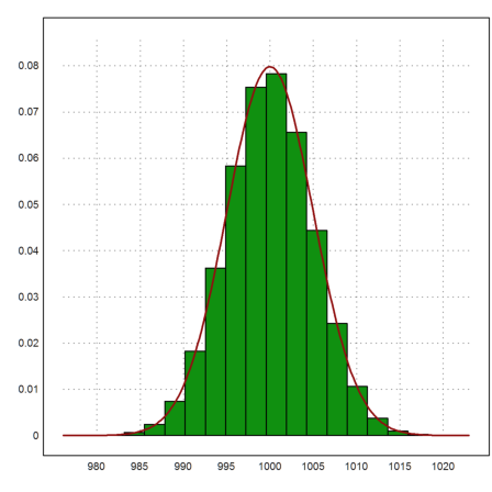
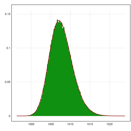
You can set the number of intervals for the distribution to 100. Then you see how closely the observed distribution and the true distribution match. After all, we have generated one million events.
>plot2d(x,distribution=100,style="#");  ...
   plot2d("qnormal(x,1000,5)",color=red,thickness=2,>add):

Of course, the mean value of these simulations and the deviation should be very close to the expected values.
>mean(x), dev(x)
999.989089709
4.99352507179
These two functions are easy to compute by elementary means. For the mean value, we can use the sum function, which takes the sum of all elements of a row vector.
>xm=sum(x)/n
999.989089709
Then the experimental deviation is the following.
>sqrt(sum((x-xm)^2/(n-1)))
4.99352507179
Note, that x-xm is a vector of corrected values, where xm is subtracted from all elements of the vector x.
Here are the first 10 values of x-xm.
>short (x-xm)[1:10]
[-1.4164,  4.1698,  3.2187,  0.92027,  3.0479,  -12.23,  2.5515,
7.0079,  2.057,  1.6789]
Using the matrix language, we can easily answer other questions. E.g., we want to compute the proportion of x which exceeds 1015.
The expression x>=1015 returns a vector of 1 and 0. Summing this vector yields the number of times x[i]>=1015 happens.
>sum(x>=1015)/n
0.00134
The expected probability of this can be computed with the normaldis(x) function. Euler uses distributions with the naming convention ...dis, so that
![]()
where X is m-s-normally distributed.
>1-normaldis(1015,1000,5)
0.00134989803163
The result should agree up to two digits with the observed frequency.
How does the >distribution flag of plot2d work? It uses the function histo(x), which produces a histogram of the frequencies of values in x. This function returns the bounds of intervals and the counts in these intervals. We normalize the counts to get frequencies.
>{t,s}=histo(x,40); plot2d(t,s/n,>bar):

The histo() function can also count the frequencies in given intervals.
>{t,s}=histo(x,v=[950,980,990,1010,1020,1050]); t, s,
[950,  980,  990,  1010,  1020,  1050]
[36,  22801,  954744,  22395,  24]
Usually, all random values will be between 950 and 1050.
>sum(s)
1000000
You can run this section again with Shift-Return. The results will be different then, because we did not set a random seed in the beginning.
To simulate 5 measurements of a normal distributed random variable, we take five 1000-5-normally distributed values a hundred thousand times.
>m=5; n=100000; A=normal(n,m)*5+1000;
The numbers are stored in the matrix A, each tupel of 5 measurements in one row. Here is the first of the 100000 rows.
>A[1]
[998.927, 989.562, 991.275, 993.44, 995.597]
Let us compute the vector of all mean values of the m measurements. Its mean value should be close to 1000.
>MA=sum(A)/m; mean(MA')
999.992749125
Note that MA is a column vector, and mean works for row vectors, just like sum and dev.
Now we can compute the vector of experimental standard deviations. We can test that the squares of these (the variations) are expected to be 5^2.
>VA=sum((A-MA)^2/(m-1)); mean(VA')
25.0305155381
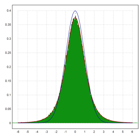
The next plot shows the distribution of
![]()
which is expected to be student-t distributed with m-1 degrees of freedom. We add the normal distribution, which is obviously only an approximate solution.
>plot2d((MA'-1000)/sqrt(VA')*sqrt(m),a=-6,b=6,c=0,d=0.4, ...
     distribution=500,style="#"); ...
   plot2d("qtdis(x,m-1)",color=red,thickness=2,>add); ...
   plot2d("qnormal(x)",color=blue,>add):
For all rows i
![]()
is chi-squared distributed with m degrees of freedom. The chi-square distribution is called chidis() in Euler, and qchidis() is its density function.
>plot2d(sum(((A-1000)/5)^2)',distribution=50);  ...
   plot2d("qchidis(x,m)",color=red,thickness=2,>add):
Using a simulation, we want to get confidence in the correctness of confidence intervals. If we have n data from a normal distributed random variable, we can estimate the mean and the standard deviation of the distribution as follows.
>n=10; x=normal(n); mean(x), dev(x),
0.128288044313
1.44395122868
Let us check these values.
>xm=sum(x)/n, xsd=sqrt(sum((x-xm)^2)/(n-1)),
0.128288044313
1.44395122868
The function cimean() returns a confidence interval for the mean value of the sampling.
>cimean(x,5%)
[-0.904652, 1.16123]
This interval should have the property that the true mean value (0 in our case) is in the interval in 95% of the cases. Using probability theory, we see that we can use the following interval.
>invtdis(0.975,n-1)*xsd/sqrt(n); [xm-%,xm+%]
[-0.904652, 1.16123]
But is this correct?
To check the correctness we simulate the procedure a lot of times.
>m=10000; X=normal(m,n); M=sum(X)/n; SD=sqrt(sum((X-M)^2/(n-1)));
We now have column matrices of means and standard deviations.
>plot2d(M',>distribution,title="Distribution of mean Values"):
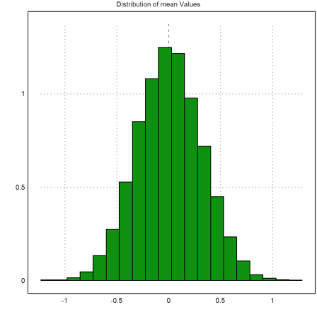
Let us compute the confidence intervals and check, how often 0 is in the interval. We get a column vector of confidence intervals.
>cf=invtdis(0.975,n-1); CI=M+cf*SD/sqrt(n)*[-1,1]; CI[1:10]
    -0.944157      0.483168
    -0.734059      0.276932
    -0.528961        1.0292
    -0.418797       1.23983
     -1.19006      0.274779
    -0.791691      0.315253
    -0.441135       1.07905
    -0.647686      0.429467
    -0.846641        1.0035
     -1.17152      0.672192
How often is 0 in these intervals? This should be close to 95%.
>sum((CI[,1]<=0 && CI[,2]>=0)')/m
0.9506
The same idea applies to the binomial distribution. If we find k hits in n independent draws, we estimate p=k/n for the probability for a single hit. We can make a confidence interval for p which is due to Clopper and Pearson.
The interval is rather large usually. For example, if we find 15 in 150 we can only say that p is between 5.7% and 16%.
>clopperpearson(15,150,5%)
[0.0570574, 0.159568]
Let us check, if this interval has the desired property. We assume that the true p is 0.12.
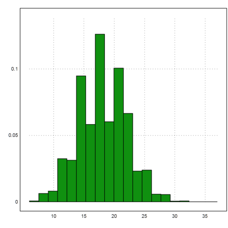
>m=10000; n=150; p=0.12; X=sum(random(m,n)<p);
Then we can plot the distribution of the number of hits. The average should be 0.12*150.
>plot2d(X',>distribution):
The function clopperpearson() does not vectorize. So we must use a loop in this case.
>CI=zeros(m,2); for k=1:m; CI[k]=clopperpearson(X[k],n,5%); end;
We count the number of times when p is in the interval in the same way as above.
>sum((p>=CI[,1] && p<=CI[,2])')/m
0.957
The distribution of the maximal value M of our measurements can be computed by the following formula.
![]()
where X is the random variable modeling one experiment. Let us try to simulate this.
>m=10; n=100000; A=normal(n,m)*5+1000;
We compute the maximal values in all rows, and then the mean value of all maximal values.
>M=max(A); mean(M')
1007.70538194
Let us test the equation above.
>sum(M'<=1010)/n, normaldis(1010,1000,5)^10
0.79286
0.794431040167
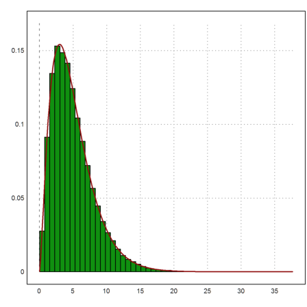
If f is the density of X and F its distribution, then F'=f, and the density of M is
![]()
We check this.
>plot2d(M',distribution=100,style="#"); ...
   plot2d("m*qnormal(x,1000,5)*normaldis(x,1000,5)^(m-1)", ...
   color=red,thickness=2,>add):
Maxima can derive the formulas in symbolic form.
>function f(x) &= 1/sqrt(2*pi)*exp(-x^2/2)
                                    2
                                   x
                                 - --
                                   2
                                E
                           ----------------
                           sqrt(2) sqrt(pi)
This is the density of the 0-1-normal distribution.
>integrate("f(x)",-10,10)
1
We derive the formula for the density of the maximal value with Maxima.
>function fM(x) &= m*f(x)*integrate(f(t),t,-inf,x)^(m-1) | factor;
Printed with "maxima: 'f[M](x) = fM(x)" we get
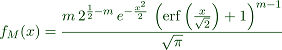
Numerically, Euler can evaluate the erf() function, which Maxima inserted into the integral.
>fM(1.5), m*qnormal(1.5)*normaldis(1.5)^(m-1)
0.695138244172
0.695138244172
We assume that the prices of assets are distributed according to
![]()
where X(dt) is some random variable, and r is a trend. E.g., the Black-Scholes model (BS-model) assumes
![]()
This is an assumption which is easy to handle but only a coarse approximation of the reality. Let us simulate this.
>T=3; n=500; dt=T/n; r=0.02; sigma=0.01;  ...
 plot2d(100*(1|cumprod(1+r*dt+sigma*sqrt(dt)*normal(10,n)))):
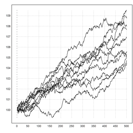
We took 500 time steps in 3 years with a volatility of 10% and an interest rate of 2%. The function cumprod() (cumulative product) just multiplies the rows from left to right.
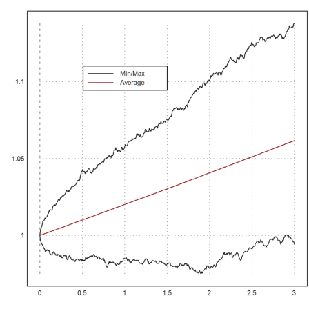
To get a better idea of the development, we take many more trajectories and plot the minimal value and the maximal value together with the mean values at times t.
>t=linspace(0,T,n); m=10000; ...
 X=1|cumprod(1+r*dt+sigma*sqrt(dt)*normal(m,n)); ...
 plot2d(t,min(X')'_max(X')'); ...
 plot2d(t,mean(X')',color=red,>add); ...
 labelbox(["Min/Max","Average"],x=0.5,y=0.2,w=0.3,colors=[black,red]):
In this simple model, the distribution of S(T) is known. It is
![]()
Let us extract the values of S(T) from our simulations and compare the mean and the variance with a direct simulation.
>v=X'[-1]; mean(v), dev(v),
1.06171178855
0.0184373618142
For the direct simulation, we can take a million points.
>vd=exp((r-sigma^2/2)*T+sigma*sqrt(T)*normal(1000000));  ...
 mean(vd), dev(vd),
1.06184051899
0.0183927533321
The expected value is exp(rT).
>exp(r*T)
1.06183654655
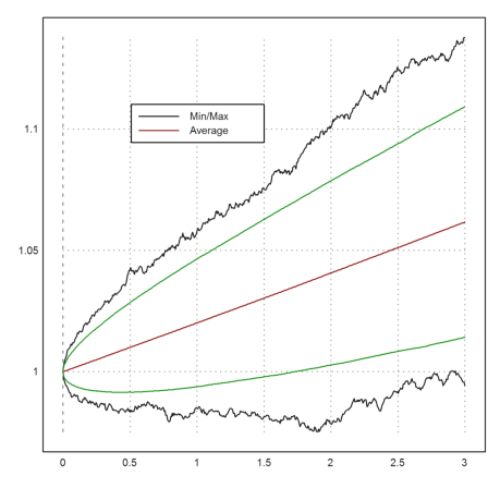
We can use our simulation to compute a vector of standard deviations depending on the time. Then we can add a 99% trust region to our plot.
>m=mean(X')'; d=dev(X')'; c=invnormaldis(0.995); ...
 plot2d(t,(m+d*c)_(m-d*c),color=green,>add):
There are tutorials for reading real stock data from the internet. There are also tutorials on the simulation of other distributions, e.g., using the rejection method.
A simple random permutation is easy to generate in Euler.
>shuffle(1:10)
[3, 8, 5, 4, 6, 9, 10, 1, 7, 2]
With that, we get lottery numbers (6 out of 49) as follows.
>sort(shuffle(1:49)[1:6])
[10, 16, 28, 42, 44, 45]
If we set a specific seed (between 0 and 1) we get lottery numbers for this day.
>seed(daynow); sort(shuffle(1:49)[1:6])
[10, 12, 30, 38, 47, 49]
To simulate a lot of random permutations, we have to use a loop. This can be done in the command line, but we make a function for it.
>function simperm (n,m) ...
 M=zeros(n,m); v=1:m;
 loop 1 to n; M[#]=shuffle(v); end;
 return M;
 endfunction
Here is an example.
>shortest simperm(10,5)
        5         2         4         3         1
        1         4         5         3         2
        5         1         4         2         3
        4         2         1         3         5
        1         4         3         5         2
        3         2         1         5         4
        1         5         3         2         4
        2         5         3         1         4
        3         5         4         2         1
        1         4         5         2         3
Now a larger example.
>A=simperm(100000,10);
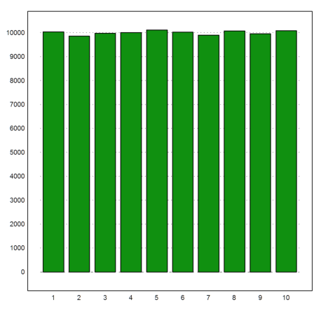
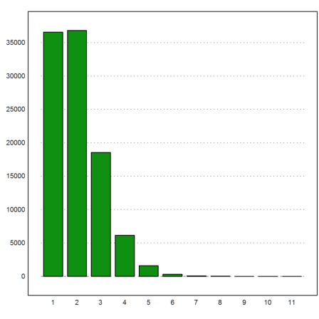
Let us count and plot the number of times each number 1 to 10 is in the first place of the permutation. For this, we can use the function getmultiplicities(x,v), which counts the number of times x is in v. We use is for x=1 to x=10.
>k=getmultiplicities(1:10,A[,1]'); columnsplot(k):
Another problem is the number of fixed points in each permutation.
We compute this in the following way. First we call A==1:10. This compares each row of A with the row vector 1:10. If A[i,j] is equal to j it stores 1, else a 0. Summing the rows yields a column number of fixed points for each row. The count is done by getmulitplicities() as above.
>kfixed=getmultiplicities(0:10,sum(A==1:10)'); columnsplot(kfixed):
Here are the relative frequencies of 0 to 10 fixed points.
>shortest kfixed/rows(A)
[0.366, 0.368, 0.186, 0.0613, 0.0159, 0.00316, 0, 0, 0, 0, 0]
It is known that the expected value of no fixed point is 1/E.
>1/E
0.367879441171
There is a simple recursion for the number of permutations of k elements, which leave exactly j elements fixed.
![]()
The reason is that with exactly j fixed elements, we have the following cases:
Counting these gives the above formula. We implement it in a simple recursive function.
>function map f(k,j) ...
 if j<0 or j>k then return 0;
 elseif k==0 and j==0 then return 1;
 else return f(k-1,j-1)+f(k-1,j)*(k-1-j)+f(k-1,j+1)*(j+1);
 endif;
 endfunction
For an effective implementation, we would need to use a matrix, which stores previously computed values.
Nevertheless, we can compute and check the probabilities for k=10.
>shortest f(10,0:10)/10!
[0.368, 0.368, 0.184, 0.0613, 0.0153, 0.00306, 0, 0, 0, 0, 0]
For j=0 there is a simple formula.
![]()
Let us check this for k=10.
>k=10; j=2:k; sum((-1)^j/j!), (kfixed/rows(A))[1]
0.367879464286
0.36568
This agrees with our observation, and it is also the reason, why this probability converges to 1/E.
>1/E
0.367879441171
Euler has a package for permutations.
>load perm.e
Functions for permutations.
With this you can multiply permutations, or enter and print permutations as cycles.
E.g., we can multiply the two cycles (1,2,3) and (2,3,4).
>pprint pcycle([1,2,3],10) pm pcycle([2,3,4],10)
(1 2)(3 4)
For our problem, we want to count the number of permutations, with exactly one fixed point.
We need the counting function first.
>function f1 (p) ...
 global k,count;
 if sum(p==1:k)==0 then count=count+1; endif;
 endfunction
Then we can use forAllPerm() to iterate through the permutations.
>k=8; count=0; forAllPerm("f1",k); count,
14833
The result is equal to the theoretical result.
>k=8; j=2:k; sum((-1)^j/j!)*k!
14833
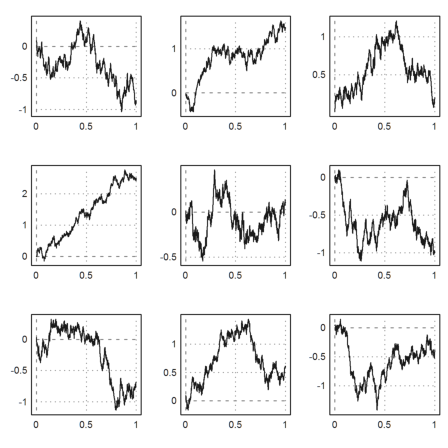
Let us try to simulate a Brownian motion.
>function args brown (n,a=0,b=1) ...
 return {linspace(a,b,n),cumsum(normal(n+1)*sqrt((b-a)/n))}
 endfunction
This function returns t-values in the range a,b and a random walk, which is 0-1-normal distributed for dt=1.
>figure(3,3); ...
 for n=1:9; figure(n); plot2d(brown(1000)); end; ...
 figure(0):
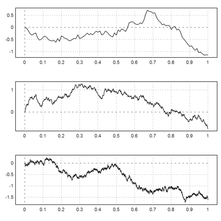
We can also demonstrate the effect of finer grids.
>figure(3,1);  ...
 for k=1:3; figure(k); plot2d(brown(10^(k+1))); end; ...
 figure(0):
Let us compute the 2-variation of such Brownian samples. It should be close to 1, independent on the grid size.
>p=2;  ...
 {x,y}=brown(1000); sum(abs(differences(y))^p)
0.958080352072
>{x,y}=brown(10000); sum(abs(differences(y))^p)
1.01110318902
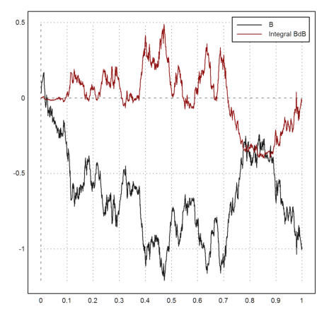
Let us try to define an "Ito-sum" for XdY.
>function ito (X,Y) ...
 return cumsum(head(X,-2)*differences(Y))
 endfunction
We apply it to the Brownian path, integrating BdB.
>{x,y}=brown(1000); z=ito(y,y); ...
 plot2d(x,y_z,style="i");  ...
 plot2d(x,y,>add);  ...
 plot2d(head(x,-2),z,>add,color=red); ...
 labelbox(["B","Integral BdB"],colors=[black,red]):