Euler Examples

Search

B-Splines

by R. Grothmann

In this notebook, we demonstrate techniques to compute such complicated things as B-splines.

First, we start with the Haar function, which is the B-spline of order 0 on a set of knots, 1 on [t[k],t[k+1]].

>function N0 (x,k,t) := x>=t[k] && x<t[k+1]

We can recursively apply the Cox formula for B-Splines.

However, we must be careful not to divide through 0. Also, we must make sure, the function works for a vector x. Since t is also a vector, we protect it from being mapped.

>function map N (x,k,n;t) ...
 ## B-Spline on t[k:k+n+1] in x.
 if n<=0 then return N0(x,k,t); endif;
 if x<=t[k] then return 0;
 else if x<t[k+n+1] then
   sum=0;
   if t[k]<t[k+n] then 
     sum=sum+N(x,k,n-1,t)*(x-t[k])/(t[k+n]-t[k]); 
   endif;
   if t[k+1]<t[k+n+1] then 
     sum=sum+N(x,k+1,n-1,t)*(t[k+n+1]-x)/(t[k+n+1]-t[k+1]); 
   endif;
   return sum;
 endif;
 return 0;
 endfunction

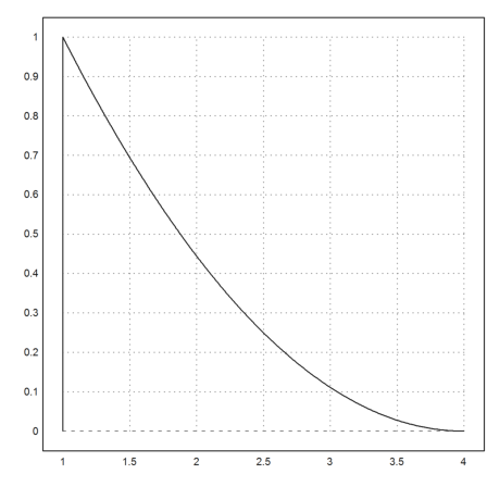
>plot2d("N";1,2,[1,2,3,4],a=1,b=4):

It does also work for multiple knots.

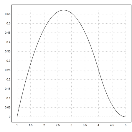
>plot2d("N";1,2,[1,1,1,4],a=1,b=4):

This function is already contained in Euler Math Toolbox. But it takes less effort and defines the spline recursively by

with a small epsilon. This avoids to check for the situation of x. The recursion formula can be applied immediately for row vectors x.

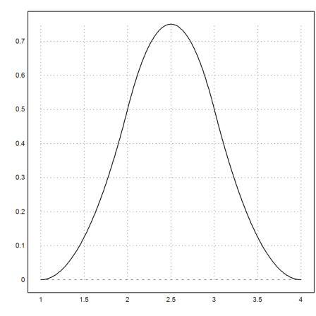
>plot2d("nspline";2,2,[1,1,1,4,5],a=1,b=5):

Let us write a function, plotting all B-Splines for a set of knots.

>function plotall (t,n) ...
 // set the plot window:
 plot2d(none,a=min(t)+epsilon,b=max(t)-epsilon,c=0,d=1);
 loop 1 to cols(t)-n-1
   plot2d("nspline";#,n,t,>add); // plot #-th B-spline
 end
 return plot();
 endfunction

>plotall([1,1,1,2,3,4,4,4],2):

The B-splines add to 1. We compute all B-splines (row 1:m) at x-values (columns) and add the columns to get the sum.

Since NSpline() does vectorize to column vectors k the matrix language can be used.

>x=0:0.01:5; t=[1,1,1,2,3.1,4,4,4]; k=1:5;  ...
 y=sum(nspline(x,k',2,t)')'; ...
 plot2d(x,y,thickness=2):

Pseudo Interpolation

We can now approximate a function f() with splines by pseudo-interpolation.

Here, the spline N[k] is the B-spline around t[k].

We first compute a matrix of B-Spline values for all a set of cubic B-Splines, which add to 1 on [0,1]. By construction, the last Spline with the knots [0.9,1,1,1,1] will be 0 in x=1. We fix that manually.

>t1=0:0.1:1; t=0|0|0|t1|1|1|1; x=0:0.01:1;  ...
 B=nspline(x,(1:cols(t)-4)',3,t); B[-1,-1]=1; ...
 plot2d(x,B,a=0,b=1.2):

The Pseudo-Interpolation has the property that the derivative is 0 in x=0 and x=1. So the direct approach here is useful only in special situations.

>function f(x) := linsplineval(x,[0,0.2,0.5,0.8,1],[1,2,1,2,1]); ...
 plot2d(x,f(x)); ...
 plot2d(x,f(t[3:cols(t)-2]).B,color=red,>add):

B-Spline Curves

Now we write a function, which computes a B-spline curve with support polygon through K (2xm or 3xm). The function will vectorize to x.

>function BSplineCurve (x,t,K) ...
 n=cols(t)-cols(K)-1;
 y=zeros(rows(K),cols(x));
 loop 1 to rows(K)
   y[#]=sum(K[#]*nsplinemap(x',1:cols(K[#]),n;t))';
 end
 return y;
 endfunction

Another function to plot the control polygon.

>function plotPolygon (K,add=1) ...
 plot2d(K[1],K[2],thickness=2,add=add);
 return plot2d(K[1],K[2],points=1,style="[]",add=1);
 endfunction

Let us test everything.

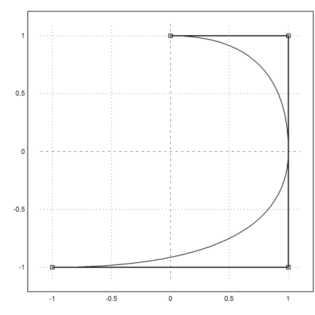
>t=[1,1,1,2,3,3,3]; K=[0,1,1,-1;1,1,-1,-1]; ...
 x=linspace(1.001,2.999,300); ...
 y=BSplineCurve(x,t,K); ...
 plot2d(y[1],y[2],a=-1.1,b=1.1,c=-1.1,d=1.1); ...
 plotPolygon(K):

Nurbs

Now, we can combine everything to compute Nurbs. We need a vector of non-zero weights. Then we can compute the three dimensional Spline and project to z=1.

>function NurbsCurve (x,t,K,w) ...
 Kw=w*K_w;
 y=BSplineCurve(x,t,Kw);
 y=y/y[3];
 return y[1:2];
 endfunction

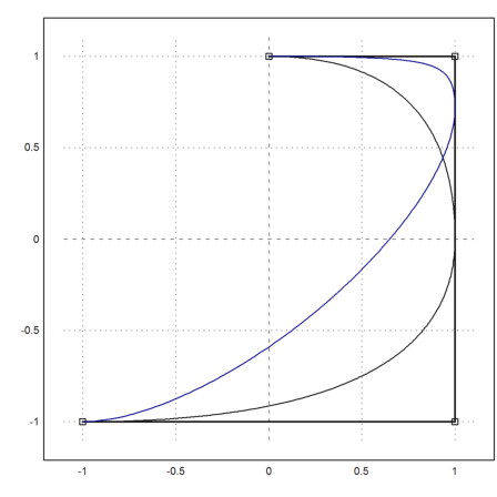
>w=[1,3,1/2,1]; y=NurbsCurve(x,t,K,w);

The nurbs are closer to the corners with higher weights.

>plot2d(y[1],y[2],add=1,color=4):

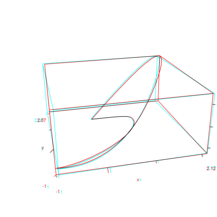
In the following anaglyph plot, we show the three dimensional weighted curve and its projection.

>y=BSplineCurve(x,t,K*w_w); h=y/y[3]; ...
 plot3d(y[1]_h[1],y[2]_h[2],y[3]_h[3], ...
   >lines,angle=-15°,>anaglyph,zoom=3.4):

Examples