by R. Grothmann
In this notebook, we use a simple algorithm proposed by Lloyd (later used by Steinhaus, MacQueen) to cluster points. The algorithm is K-Means-Clustering. Clustering can be used to classify data for data mining.
>load clustering;
To generate some nice data, we take three points in the plane.
>m=3*normal(3,2);
Now we spread 100 points randomly around these points.
>x=m[intrandom(1,100,3)]+normal(100,2);
Now we have a matrix of 100 points with two columns.
>size(x)
[100, 2]
We want three clusters.
>k=3;
The function kmeanscluster() contains the algorithm. It returns the indices of the clusters the points contain to.
>j=kmeanscluster(x,k);
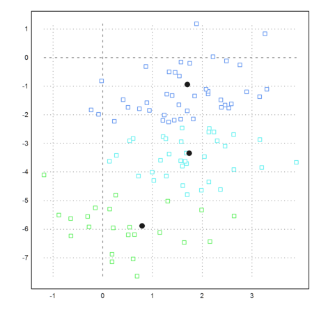
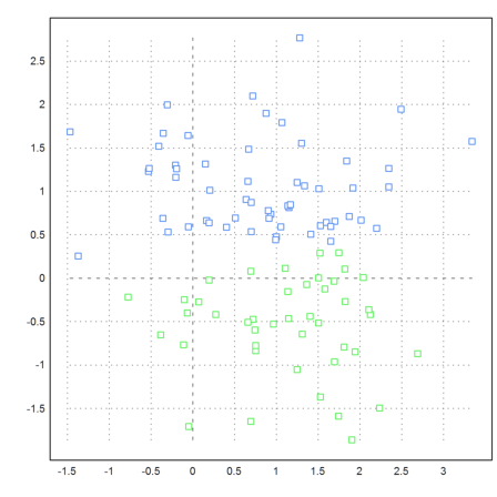
We plot each point with a color representing its cluster.
>P=x'; plot2d(P[1],P[2],color=10+j,points=1); ...
We add the original cluster centers to the plot.
>loop 1 to k; plot2d(m[#,1],m[#,2],points=1,style="o#",add=1); end; ...
 insimg;
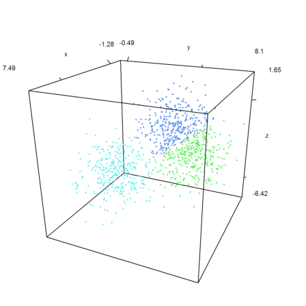
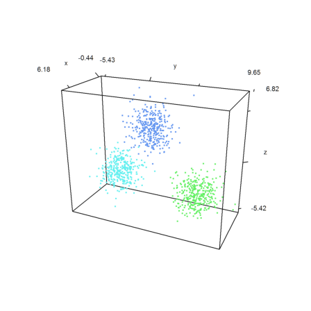
The same in 3D.
>k=3; m=3*normal(k,3); ...
 x=m[intrandom(1,1000,k)]+normal(1000,3); ...
 j=kmeanscluster(x,k); ...
 P=x'; plot3d(P[1],P[2],P[3],color=10+j,>points,style=".."); ...
   insimg();
The file clustring.e contains another clustering algorithm.
This algorithm uses a clustering of the elements of the eigenvector to the k largest eigenvalues of a similarity matrix. The similarity matrix is derived from the distance matrix.
>k=2; m=normal(2,2); ...
 x=m[intrandom(1,100,k)]+normal(100,2); ...
 j=eigencluster(x,k); ...
 P=x'; plot2d(P[1],P[2],color=10+j,points=3):
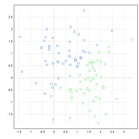
For comparison, the k-means clustering.
>j=kmeanscluster(x,k); ...
 P=x'; plot2d(P[1],P[2],color=10+j,points=1):
Here is another example.
Clearly, the algorithm with eigenvalues takes a much larger effort. However, this could be removed by Krylov-Methods. As implemented, the algorithms uses the Jacobi method.
>k=3; m=3*normal(k,3); ...
 x=m[intrandom(1,1000,k)]+normal(1000,3); ...
 j=eigencluster(x,k); ...
 P=x'; plot3d(P[1],P[2],P[3],color=10+j,>points,style=".."):

K-Means-Clustering is a lot faster.
>j=kmeanscluster(x,k); ...
 P=x'; plot3d(P[1],P[2],P[3],color=10+j,>points,style=".."):
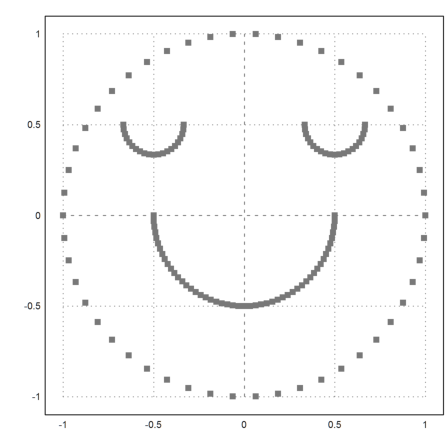
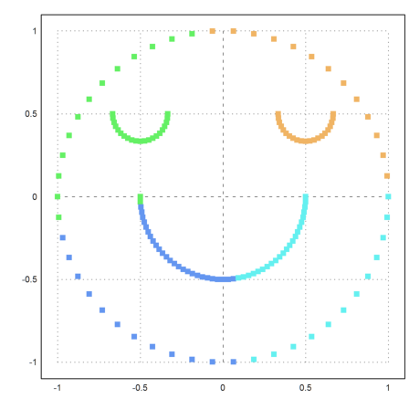
If you look at the following example you see that clustering is based on the distance of points. We define a set of points, which is easy to cluster visually.
>t=linspace(0,2pi,50)'; x=cos(t); y=sin(t); ...
 t=linspace(pi,2pi,50)'; x=x_cos(t)/2; y=y_sin(t)/2; ...
 t=linspace(pi,2pi,20)'; x=x_(0.5+cos(t)/6); y=y_(0.5+sin(t)/6); ...
 x=x_(-0.5+cos(t)/6); y=y_(0.5+sin(t)/6); ...
 X=x|y; ...
 P=X'; plot2d(P[1],P[2],>points,style="[]#",color=gray):
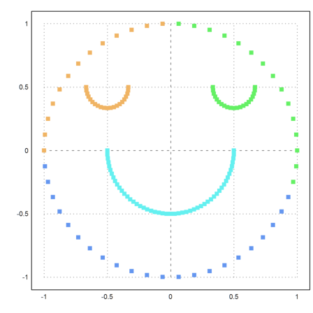
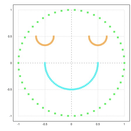
But the function eigencluster() defines a very special similarity matrix. This makes the example work relatively well.
>j=eigencluster(X,4); ...
 P=X'; plot2d(P[1],P[2],color=10+j,>points,style="[]#"):
The function kmeanscluser() uses simple distances and does not work so well here.
>j=kmeanscluster(X,4); ...
 plot2d(P[1],P[2],color=10+j,>points,style="[]#"):
How could we improve the result. We need to compute the distances of the point in some other way.
First we write a function to compute the distances of m points in m rows of a mxn matrix.
>function distances (X) ...
 P=X';
 S=(P[1]-P[1]')^2;
 loop 2 to cols(X); S=S+(P[#]-P[#]')^2; end;
 return sqrt(S);
 endfunction
Now we use another difference function. We define
![]()
This is the minimal hop we would have to make if we travelled from A to B.
To compute this, we take the minimum over k=2, k=4, k=8 etc. points. So we need to apply the minimization algorithm log(m) times.
>function improve (S) ...
 S=S;
 loop 1 to log(rows(S))/log(2)+4
   loop 1 to rows(S)
     S[#]=min(max(S[#],S))';
   end;
   S=min(S,S');
 end;
 return S;
 endfunction
The symmetry matrix used by the eigenvalue matrix is the following. This is from the theory of eigenvalue clustering.
>function simmatrix (S) ...
   D=sqrt(sum(S));
   S=exp(-((S/D)/D')^2); D=sqrt(sum(S));
   return id(cols(S))-(S/D)/D';
 endfunction
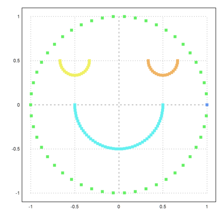
The result is better, but only three clusters are found.
>S=simmatrix(improve(distances(X))); ...
 j=similaritycluster(S,4); ...
 plot2d(P[1],P[2],color=10+j,>points,style="[]#"):
It helps to force 5 clusters. But then we get an extra cluster consisting of one point.
>j=similaritycluster(S,5); ...
 plot2d(P[1],P[2],color=10+j,>points,style="[]#"):
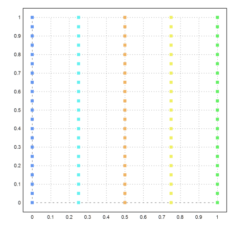
Here is another example, where k-means clustering does not work well.
>{x,y}=field(0:0.25:1,0:0.05:1); n=prod(size(x)); ...
 X=redim(x,n,1)|redim(y,n,1); ...
 j=kmeanscluster(X,5); ...
 P=X'; plot2d(P[1],P[2],color=10+j,>points,style="[]#"):
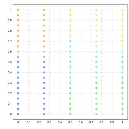
Let us try our new method. This time, it turns out perfect.
>S=simmatrix(improve(distances(X))); ...
 j=similaritycluster(S,5); ...
 plot2d(P[1],P[2],color=10+j,>points,style="[]#"):